Sparse Autoencoders Find Highly Interpretable Features in Language Models
arXiv:2309.08600 · PDF · 20 pp. · its place among the papers
One paper, several tellings. The big picture states the paper’s own thesis and contributions in its own terms; Inside the paper follows the paper’s own arc; Across the corpus traces how it connects to the other papers; The concepts lists everything the paper uses, in reading order. The experiments explains the paper’s experiments and results as one connected account, built from the paper’s concepts, with its figures and tables attached as supporting evidence — each opening into a page of its own. Pick a tab, then use the +/− toggles to open it level by level, or set a granularity to read the whole thing at that zoom.
Strip away the corpus and the citations, and this paper makes one claim in its own words: individual neurons are the wrong place to look for what a language model represents, because a network can pack more concepts than it has neurons by scattering them across shared, overlapping directions instead of clean, separate units.
What follows is the paper's own argument, in its own vocabulary: the thesis that neurons hide more than they show, the autoencoder built to recover the directions underneath them, the evidence that the recovered features score and localize better than every rival decomposition tried, a demonstration on two individual features examined by hand, and the limits the paper reports against its own result.
Read at
The 2023 argument: neurons are the wrong unit, and a learned dictionary is the fix (5 chapters)
Evidence for the thesis runs in three stages: the theoretical case that superposition, not just noisy training, is why individual neurons are polysemantic; the autoencoder built to recover the overcomplete set of directions superposition implies; and two kinds of proof that the recovered features are genuinely better than four rival decompositions, an automated interpretability score run at scale and a causal-patching test on a well-understood behavior, backed up by two individual features examined by hand. The paper reports its own limits alongside the result: reconstruction that never reaches zero, a recipe that partly breaks on MLP activations, and a safety ambition it names as unreached.
Chapter 1The thesis: neurons hide more than they show (5 concepts)
The paper's central claim, stated in its abstract and defended for the rest of its length, is that polysemanticity — individual neurons activating in multiple, semantically distinct contexts — is caused by superposition, models representing more features than they have neurons by assigning them to an overcomplete set of directions rather than to individual neurons. Sparse autoencoders are offered as a scalable, unsupervised method for recovering those directions directly, aimed at providing “a foundation for future mechanistic interpretability work.”
Why a network can represent more than it has room for concept (2 connections)
A hypothesized cause of polysemanticity in which a network represents more features than it has dimensions by assigning them to an overcomplete set of non-orthogonal directions, relying on activation sparsity to limit interference between them. The paper's stated goal is to resolve superposition in language models directly, by recovering these directions via sparse dictionary learning rather than working around the problem.
connections
- Superposition — manifests as → Polysemanticity
- Superposition — motivates → Sparse autoencoders (SAEs)
The opening problem the whole paper answers to concept (2 connections)
The paper's opening problem: individual neurons activate in multiple, semantically unrelated contexts, preventing concise, human-understandable explanations of what a network is doing internally. Named in the abstract's first sentence as “one of the roadblocks to a better understanding of neural networks' internals,” it is the roadblock the paper's entire method is aimed at removing.
connections
- Polysemanticity — blocks → Mechanistic interpretability
- Superposition — manifests as → Polysemanticity
The property the recovered directions are judged by concept (3 connections)
The property the method is judged by: a feature activating for a single, coherent, human-interpretable concept, the converse of polysemanticity. The paper's case studies — an apostrophe-detecting feature and a closing-parenthesis-predicting feature — are framed as demonstrating that learned dictionary features are highly monosemantic compared to neurons or other baseline directions, even if not every feature covers an entire human-nameable category on its own.
connections
- Apostrophe dictionary feature (feature 556) — demonstrates the limits of → Monosemanticity
- Monosemanticity — is imperfectly proxied by → Autointerpretability score
- Monosemanticity — benchmarks → Dictionary feature
The discipline the method is offered to advance concept (2 connections)
The research agenda the paper names as its home discipline: reverse-engineering a network's internal computations well enough to make targeted changes to them, motivated in part by the worry that AI systems might deceive humans to accomplish undesirable goals. The paper offers its method as “a foundation for future mechanistic interpretability work,” hoping it will “enable greater model transparency and steerability.”
connections
- Mechanistic interpretability — is the field that dreams of → Enumerative safety
- Polysemanticity — blocks → Mechanistic interpretability
The method: an autoencoder built to unmix superposition concept (14 connections)
The paper's method: a single-hidden-layer, ReLU, tied-weight autoencoder trained with an L1 sparsity penalty to reconstruct a language model's activations as a sparse linear combination of an overcomplete dictionary of learned features. The paper's central claim about this object is that the resulting features are more interpretable, more monosemantic, and more causally precise than neurons or any of four alternative decompositions tested.
connections
- Default (neuron/residual-stream) basis baseline — loses to → Sparse autoencoders (SAEs)
- Sparse autoencoders (SAEs) — is framed as a step toward → Enumerative safety
- Independent Component Analysis (ICA) — converges with → Sparse autoencoders (SAEs)
- Principal Component Analysis (PCA) — trails → Sparse autoencoders (SAEs)
- Sparse autoencoders (SAEs) — runs counter to the depth profile of → Residual stream hindsight
- SAE decomposition of persona vectors — applies the unsupervised machinery of → Sparse autoencoders (SAEs)
- SAE training on the MLP sublayer — stress tests → Sparse autoencoders (SAEs)
- Sharkey et al. (2023) interim research report — is validated at scale by → Sparse autoencoders (SAEs)
- Sparse dictionary learning / sparse coding — operationalized as → Sparse autoencoders (SAEs)
- Sparsity-reconstruction tradeoff (no single correct decomposition) — rules out a single canonical dictionary for → Sparse autoencoders (SAEs)
- Sparse autoencoders (SAEs) — offers an unsupervised alternative to → Steering vector hindsight
- Superposition — motivates → Sparse autoencoders (SAEs)
- Tied encoder/decoder weights — is the default configuration of → Sparse autoencoders (SAEs)
- Transformer visualization via dictionary learning (Yun et al., 2021) — is extended by → Sparse autoencoders (SAEs)
Chapter 2The method: sparsity traded against reconstruction (4 concepts)
Building the dictionary means committing to a single training objective with two competing terms: reconstruct the original activation as closely as possible, while keeping the code that reconstructs it as sparse as possible. Every other design choice in the method — how overcomplete the dictionary is, how its weights are structured — is downstream of how that one tradeoff is set.
The central unit: one learned direction concept (5 connections)
A single learned row of the autoencoder's weight matrix, representing one direction in activation space used to reconstruct inputs as part of a sparse linear combination. Individual dictionary features are the paper's central unit of analysis throughout — examined for interpretability, causal importance, and monosemanticity in turn.
connections
- Dictionary feature — scores unevenly across depth in → Autointerpretability score
- Dead features — hollows out the count of → Dictionary feature
- L4-norm maximization (sparse dictionary search reformulation) — predicts the heavy tailed activation of → Dictionary feature
- Monosemanticity — benchmarks → Dictionary feature
- Sparsity loss (L1 penalty on feature activations) — forces unit norm on → Dictionary feature
The penalty that keeps the code sparse concept (2 connections)
The L1 penalty on the autoencoder's hidden-layer coefficients, encouraging each activation to be reconstructed from as few active features as possible. The sparsity coefficient is the paper's key hyperparameter, swept throughout every experiment to trade sparsity against reconstruction accuracy rather than fixed at one value.
connections
- Sparsity loss (L1 penalty on feature activations) — forces unit norm on → Dictionary feature
- Sparsity loss (L1 penalty on feature activations) — trades off against → Reconstruction loss
The term that admits the dictionary is incomplete concept (2 connections)
The squared-error term measuring how well the autoencoder's output matches the original activation it was given. The paper is explicit that this loss never reaches zero in its experiments — the dictionary does not capture everything a layer's activations carry, a gap the paper treats as an open limitation rather than something the method has yet resolved.
connections
- Reconstruction-substitution perplexity metric — independently corroborates → Reconstruction loss
- Sparsity loss (L1 penalty on feature activations) — trades off against → Reconstruction loss
The dial that sets how overcomplete the dictionary is concept (2 connections)
The hyperparameter controlling how overcomplete the learned dictionary is, the ratio between the autoencoder's hidden dimension and the model's own activation dimension. The paper finds interpretability gains hold even for undercomplete dictionaries, with larger dictionaries simply explaining more of a layer's overall activation variance rather than producing individually more interpretable features.
connections
- Dictionary expansion factor (R) — governs emergence of → Dead features
- Dictionary expansion factor (R) — sets the operating point on → Sparsity-reconstruction tradeoff (no single correct decomposition)
Chapter 3The evidence: features that score and localize better than every alternative (5 concepts)
Two experiments carry the paper's argument that its dictionary features are not just plausible but genuinely superior. An automated scoring pipeline, run across thousands of features, measures interpretability against four baseline decompositions; a causal-patching test on a well-understood model behavior checks whether the winning features do anything at all, not just whether they look interpretable.
The scoring pipeline: explain, then simulate concept (9 connections)
The paper's primary interpretability measure: a language model is shown text where a feature activates and writes a natural-language explanation, then a second model uses that explanation alone to predict the feature's activations on held-out text, with the correlation between predicted and actual activations as the score. Run across thousands of features, dictionary features score higher on average than every one of the paper's four baseline decompositions.
connections
- Dictionary feature — scores unevenly across depth in → Autointerpretability score
- GPT-3.5 — simulates activations for → Autointerpretability score
- GPT-4 — generates explanations for → Autointerpretability score
- Interpretability-vs-kurtosis/skew correlation analysis — explains variation in → Autointerpretability score
- Monosemanticity — is imperfectly proxied by → Autointerpretability score
- Autointerpretability score — prefigures the llm judge pattern of → Open-ended generation evaluation with GPT-4 rating hindsight
- Random directions baseline — anchors → Autointerpretability score
- Reconstruction-substitution perplexity metric — measures a different axis than → Autointerpretability score
- Top-and-random vs. random-only interpretability scoring — shapes fragment sampling in → Autointerpretability score
The baseline that loses once causal precision is what's tested concept (3 connections)
One of four baseline decompositions the paper's dictionary features are measured against. On the causal-localization test, PCA needs more patched components and larger edit magnitude than the dictionary to reach a given level of behavioral change — a gap the paper traces specifically to its sparsity penalty, since removing that penalty from the same architecture erases the advantage entirely.
connections
- Principal Component Analysis (PCA) — gets more training data than → Independent Component Analysis (ICA)
- Principal Component Analysis (PCA) — is the projection technique behind → PCA visualization of contrastive activations
- Principal Component Analysis (PCA) — trails → Sparse autoencoders (SAEs)
The naive baseline: just read the coordinates directly concept (3 connections)
The naive baseline of treating individual neurons, or individual residual-stream coordinates, as the unit of analysis. The paper's apostrophe case study makes the comparison direct: the best-matching raw coordinate the paper could find is still polysemantic across much of its activation range, where the matched dictionary feature stays clean throughout.
connections
- Apostrophe dictionary feature (feature 556) — is benchmarked against → Default (neuron/residual-stream) basis baseline
- Outlier dimensions — fails to elevate → Default (neuron/residual-stream) basis baseline
- Default (neuron/residual-stream) basis baseline — loses to → Sparse autoencoders (SAEs)
The causal test: patch a feature, and measure what moves concept (3 connections)
The paper's causal test: run the model on a counterfactual sentence, cache the resulting feature activations, then add the encoded differences for a chosen subset of features back into a base sentence's residual stream, measuring how far the output moves toward the counterfactual target. This reaches a given level of change using fewer patched features and a smaller edit magnitude than an equivalent patch built from PCA components.
connections
- Activation patching — is adapted into → Dictionary-feature patching procedure
- Dictionary-feature patching procedure — is tested against → Indirect Object Identification (IOI) task
- Less-than-rank-one ablation — edits with finer granularity than → Dictionary-feature patching procedure
The behavior used to test causal precision concept (1 connection)
The behavior used to test causal precision: a model correctly naming the recipient in sentences like “Alice and Bob went to the store. Alice gave a snack to ___.” Its circuit was already well-understood externally before this paper touched it, which is what lets the paper confirm that the features its patching procedure identifies as important are actually the ones responsible for the behavior.
connections
- Dictionary-feature patching procedure — is tested against → Indirect Object Identification (IOI) task
Chapter 4The demonstration: two features, read from both ends (3 concepts)
Aggregate scores establish that dictionary features are interpretable on average; two hand-picked features establish what that interpretability actually looks like up close. One is examined for what activates it and what it causes; the other is examined for what causes it.
A feature that fires on apostrophes, and only apostrophes concept (3 connections)
A feature that activates almost exclusively on apostrophe tokens, the paper's central worked example of monosemanticity. Ablating it specifically suppresses the model's prediction of the following 's' token, giving it an intuitive, predictable effect on the model's output — in clear contrast to the polysemantic raw coordinate that shares its top activations.
connections
- Apostrophe dictionary feature (feature 556) — divides case study labor with → Closing-parenthesis dictionary feature
- Apostrophe dictionary feature (feature 556) — is benchmarked against → Default (neuron/residual-stream) basis baseline
- Apostrophe dictionary feature (feature 556) — demonstrates the limits of → Monosemanticity
A feature whose own weights nearly name its meaning concept (2 connections)
A feature in the model's final layer whose unembedding directly predicts closing-parenthesis tokens — a meaning confirmable almost without any activation data at all, since a final-layer feature's unembedding directly names the tokens it promotes. Its near-unambiguous identity is what makes it a credible test case for the paper's circuit-tracing method.
connections
- Apostrophe dictionary feature (feature 556) — divides case study labor with → Closing-parenthesis dictionary feature
- Closing-parenthesis dictionary feature — seeds → Automatic feature circuit detection
Tracing a feature back to what causes it concept (4 connections)
A method for tracing which upstream features cause a target feature to activate: sample contexts where the target fires, ablate each candidate upstream feature in turn, and rank candidates by how much their removal lowers the target's activation. Applied to the closing-parenthesis feature, it surfaces upstream features detecting dates, acronyms, and other parenthesis-preceding phrases — an interpretable, sensible-looking circuit built from nothing but repeated ablation.
connections
- Automated Circuit Discovery (ACDC) — lends its ranking logic to → Automatic feature circuit detection
- Closing-parenthesis dictionary feature — seeds → Automatic feature circuit detection
- Automatic feature circuit detection — is offered as a concrete step toward → Enumerative safety
- Weight-based feature connection attempt (failed method) — is the failed precursor to → Automatic feature circuit detection
Chapter 5The limits the paper names against its own result (3 concepts)
The paper closes by naming exactly where its own method stops working, rather than letting the interpretability and causal-precision results stand unqualified. Reconstruction never fully succeeds, the recipe validated on the residual stream breaks down when ported to MLP activations, and the safety ambition the method is offered toward is explicitly named as unreached.
A modest-looking loss, made concrete concept (2 connections)
A check on how much information the dictionary actually loses: substitute a layer's activations with the autoencoder's reconstruction and measure the resulting rise in the model's perplexity. For one tested layer, this raises perplexity from 25 to 40, nearly doubling it — concrete evidence that a reconstruction loss which looks small in the abstract still costs the model real predictive accuracy.
connections
- Reconstruction-substitution perplexity metric — measures a different axis than → Autointerpretability score
- Reconstruction-substitution perplexity metric — independently corroborates → Reconstruction loss
The recipe, ported to a harder setting, and half-breaking concept (3 connections)
An attempt to extend the method from the residual stream to MLP sublayer activations, reported as “mixed success”: many resulting features are more interpretable than individual neurons, but the approach suffers from large numbers of features that never activate at all, and does not yet reliably learn an overcomplete dictionary in the model's middle or later MLP layers.
connections
- SAE training on the MLP sublayer — confronts → Privileged basis
- SAE training on the MLP sublayer — stress tests → Sparse autoencoders (SAEs)
- Tied encoder/decoder weights — gives way to an untied variant in → SAE training on the MLP sublayer
The ambition the paper admits it has not reached concept (3 connections)
The long-term goal the paper names in its conclusion: a complete, human-understandable enumeration of a model's features, sufficient to guarantee it will not perform dangerous behaviors such as deception. The paper is explicit that it offers only “a step towards” this ambition, not an instance of it — reconstruction never reaches zero, MLP dictionaries lose many features, and only a handful of layers on two small models have been tested.
connections
- Automatic feature circuit detection — is offered as a concrete step toward → Enumerative safety
- Mechanistic interpretability — is the field that dreams of → Enumerative safety
- Sparse autoencoders (SAEs) — is framed as a step toward → Enumerative safety
A language model's individual neurons rarely mean just one thing: the same neuron can fire for several unrelated concepts at once, with no reliable way to tell from the outside which one is driving it. That makes reverse-engineering a network's behavior nearly hopeless if neurons are the unit you are stuck reading. This 2023 paper argues neurons were never the right unit to look at, and builds a small autoencoder that finds units that are.
What follows tracks the paper's own path through Pythia's residual stream: the theoretical case that models pack more concepts than they have neurons, the autoencoder built to unpack them, the automated scoring that checks whether the unpacking actually helps, the causal test that checks whether the resulting features do anything, two features examined by hand, and the limits the paper names against its own method.
Read at
Inside Sparse Autoencoders: neurons give way to a learned dictionary of directions (7 chapters)
The paper's own arc runs from a diagnosis to an instrument to three kinds of proof: why neurons and superposition make the model's internals illegible, how a small autoencoder trained with an L1 penalty is built to unpack them, how an automated scoring pipeline checks whether the unpacking beats four rival decompositions, how a causal patching test on a known behavior checks whether the resulting features actually do anything, how two hand-picked features hold up when read from both ends, and where the method's own reconstruction gap, MLP struggles, and safety ambition are left honestly unresolved.
Chapter 1The obstacle: superposition, and why neurons are the wrong unit (7 sections)
The introduction states the paper's target directly: polysemanticity, individual neurons activating for multiple unrelated concepts, is “one of the roadblocks to a better understanding of neural networks' internals” (sparse-autoencoders, Abstract, p. 1). Superposition is offered as the hypothesized cause — models packing more features than they have neurons into an overcomplete set of directions — which reframes the problem as sparse dictionary learning, a decades-old framework this paper's introduction traces from Olshausen & Field's 1997 sparse coding through a 2023 interim report by one of its own co-authors.
The roadblock named in the first sentence concept (2 connections)
Polysemanticity is named in the paper's opening sentence as the roadblock motivating everything that follows: neurons “appear to activate in multiple, semantically distinct contexts,” which “prevents us from identifying concise, human-understandable explanations for what neural networks are doing internally” (sparse-autoencoders, Abstract, p. 1). Using individual neurons as the unit of analysis “has had some success,” the paper concedes, but polysemanticity is the specific failure mode that success runs into.
connections
- Polysemanticity — blocks → Mechanistic interpretability
- Superposition — manifests as → Polysemanticity
The hypothesized cause the method is built to reverse concept (2 connections)
Superposition is the hypothesized mechanism behind polysemanticity: a network represents more features than it has dimensions by assigning them to an overcomplete set of non-orthogonal directions, relying on sparse activation to keep interference between them manageable. “Without high sparsity, interference between non-orthogonal features prevents any performance gain from superposition” (sparse-autoencoders, §1 Introduction, p. 1) — the paper's stated goal is to resolve superposition by recovering those directions directly.
connections
- Superposition — manifests as → Polysemanticity
- Superposition — motivates → Sparse autoencoders (SAEs)
The converse property the method is judged by concept (3 connections)
Monosemanticity is the converse property the paper's method is built to find: a feature or direction that activates for one coherent, human-interpretable concept rather than several unrelated ones. It becomes a demonstrated, not just scored, property once the apostrophe and closing-parenthesis case studies (Section 5) show individual dictionary features behaving this way under direct hand inspection.
connections
- Apostrophe dictionary feature (feature 556) — demonstrates the limits of → Monosemanticity
- Monosemanticity — is imperfectly proxied by → Autointerpretability score
- Monosemanticity — benchmarks → Dictionary feature
The field this method is offered to advance concept (2 connections)
Mechanistic interpretability is named as the field this method aims to advance: a research agenda seeking to “reverse engineer parts of [a network's] internal processes and make targeted changes to them,” motivated in part by the worry that AI systems “might deceive humans in order to accomplish undesirable goals” (sparse-autoencoders, §1 Introduction, p. 1). The paper positions its method as “a foundation for future mechanistic interpretability work.”
connections
- Mechanistic interpretability — is the field that dreams of → Enumerative safety
- Polysemanticity — blocks → Mechanistic interpretability
The decades-old framework the problem reduces to concept (3 connections)
Sparse dictionary learning is the decades-old mathematical framework, developed by Olshausen & Field (1997) and Lee et al. (2006) to model sparse coding in the visual cortex, that the introduction identifies its problem with: finding features is “equivalent to the well-known problem of sparse dictionary learning.” The paper's sparse autoencoder is presented throughout as a scalable neural-network implementation of that older framework, applied here for the first time at this scale to language-model activations.
connections
- Interpretability-vs-kurtosis/skew correlation analysis — supplies empirical evidence for → Sparse dictionary learning / sparse coding
- L4-norm maximization (sparse dictionary search reformulation) — reformulates → Sparse dictionary learning / sparse coding
- Sparse dictionary learning / sparse coding — operationalized as → Sparse autoencoders (SAEs)
The direct predecessor, co-authored by the same person concept (1 connection)
Sharkey, Braun & Millidge's 2023 unpublished interim report, titled “Taking features out of superposition with sparse autoencoders” — the exact phrase this paper's Section 2 heading borrows — first proposed training sparse autoencoders on language model activations and showed in toy settings that the idea could recover known ground-truth features. This paper, co-authored by Lee Sharkey himself, is explicitly framed as scaling that report up to a real language model and adding the autointerpretability, causal-localization, and monosemanticity evaluations it lacked.
connections
- Sharkey et al. (2023) interim research report — is validated at scale by → Sparse autoencoders (SAEs)
A lineage running from 1997 to a co-author's own 2023 report theme (4 concepts)
The paper presents its method as a scaling-up of existing ideas rather than a new invention: sparse dictionary learning itself traces to Sparse dictionary learning / sparse coding's decades-old sparse-coding framework, Transformer visualization via dictionary learning (Yun et al., 2021) already applied a version of it to every residual-stream layer of a transformer at once, and L4-norm maximization (sparse dictionary search reformulation) supplies a separate theoretical reformulation the paper later invokes to explain why interpretability correlates with how heavy-tailed a feature's activations are. Read together, this lineage runs from a 1997 optimization principle through a 2021 transformer-scale precedent to a co-author's own unpublished 2023 forerunner.
Sparse dictionary learning / sparse coding (3 connections)
- Interpretability-vs-kurtosis/skew correlation analysis — supplies empirical evidence for → Sparse dictionary learning / sparse coding
- L4-norm maximization (sparse dictionary search reformulation) — reformulates → Sparse dictionary learning / sparse coding
- Sparse dictionary learning / sparse coding — operationalized as → Sparse autoencoders (SAEs)
Sparse dictionary learning, also called sparse coding, is the decades-old mathematical framework Cunningham et al. (2023) build on rather than invent: Olshausen and Field (1997) and Lee et al. (2006) developed it to model how the visual cortex represents natural images, expressing each data vector as a sparse linear combination of an overcomplete set of learned basis vectors, a dictionary. The paper's sparse autoencoder is presented as a scalable neural-network implementation of this same framework, applied to language-model activations instead of images. Two more recent papers bring the framework specifically to transformers, starting with Yun et al. (2021).
Transformer visualization via dictionary learning (Yun et al., 2021) (1 connection)
- Transformer visualization via dictionary learning (Yun et al., 2021) — is extended by → Sparse autoencoders (SAEs)
Yun et al. (2021) apply sparse dictionary learning to the residual-stream activations of a language model across all its layers simultaneously, framing each token's representation as a linear superposition of shared 'transformer factors.' Cunningham et al. (2023) cite it as closely related prior work, applying a similar technique but without the interpretability and causal-localization evaluations -- autointerpretability scoring, IOI-patching precision -- that this paper contributes. A second, unpublished predecessor supplies the more direct line to this paper's specific method.
Sharkey et al. (2023) interim research report (1 connection)
- Sharkey et al. (2023) interim research report — is validated at scale by → Sparse autoencoders (SAEs)
Sharkey, Braun, and Millidge's (2023) unpublished interim research report, 'Taking features out of superposition with sparse autoencoders,' is the paper Cunningham et al. (2023) name as their direct motivation: it first proposed training sparse autoencoders specifically on language-model activations to address superposition, the idea this paper scales up with systematic evaluation. Where Yun et al. contributes a related technique, Sharkey et al. contributes the framing this paper is built to test -- sparse autoencoders as a tool for resolving superposition. A separate theoretical result, unconnected to either predecessor, explains one of this paper's own findings about which features turn out interpretable.
L4-norm maximization (sparse dictionary search reformulation) (2 connections)
- L4-norm maximization (sparse dictionary search reformulation) — predicts the heavy tailed activation of → Dictionary feature
- L4-norm maximization (sparse dictionary search reformulation) — reformulates → Sparse dictionary learning / sparse coding
L4-norm maximization is a prior theoretical result (Qu et al., 2019) showing that searching for a sparse, overcomplete dictionary can be reformulated as searching for directions that maximize the L4 norm, a measure of how heavy-tailed a distribution is. Cunningham et al. (2023) invoke it to explain their finding that a feature's autointerpretability score correlates, weakly but consistently, with the skew and kurtosis of its activation distribution (0.19 and 0.24 respectively). It also explains why Independent Component Analysis, which directly maximizes non-Gaussianity, is the strongest of the paper's non-dictionary-learning baselines -- closing the lineage from decades-old theory about the visual cortex to a specific number reported in this paper's own results.
Chapter 2The instrument: an autoencoder that trades sparsity for reconstruction (8 sections)
Section 2 lays out the recipe: a single-hidden-layer, ReLU, tied-weight autoencoder is trained to reconstruct a language model's activations from a sparse code, with the encoder c = ReLU(Mx+b) producing that code in one forward pass rather than re-solving a fresh optimization per datapoint the way classical sparse coding would. Every design choice in the section is a position on one tradeoff, set most directly by the training objective's two loss terms and the dictionary-size hyperparameter governing how overcomplete the hidden layer is allowed to be.
The method itself: an autoencoder built to unmix superposition concept (14 connections)
A sparse autoencoder, in this paper's design, is a single-hidden-layer, ReLU, tied-weight network trained with an L1 penalty on its hidden activations to reconstruct a language model's activations as a sparse linear combination of an overcomplete dictionary. It is one of two founding empirical demonstrations, alongside the concurrent Anthropic “Towards Monosemanticity” work, that this architecture recovers features more interpretable and monosemantic than PCA, ICA, or the neuron basis (sparse-autoencoders, §2, p. 2).
connections
- Default (neuron/residual-stream) basis baseline — loses to → Sparse autoencoders (SAEs)
- Sparse autoencoders (SAEs) — is framed as a step toward → Enumerative safety
- Independent Component Analysis (ICA) — converges with → Sparse autoencoders (SAEs)
- Principal Component Analysis (PCA) — trails → Sparse autoencoders (SAEs)
- Sparse autoencoders (SAEs) — runs counter to the depth profile of → Residual stream hindsight
- SAE decomposition of persona vectors — applies the unsupervised machinery of → Sparse autoencoders (SAEs)
- SAE training on the MLP sublayer — stress tests → Sparse autoencoders (SAEs)
- Sharkey et al. (2023) interim research report — is validated at scale by → Sparse autoencoders (SAEs)
- Sparse dictionary learning / sparse coding — operationalized as → Sparse autoencoders (SAEs)
- Sparsity-reconstruction tradeoff (no single correct decomposition) — rules out a single canonical dictionary for → Sparse autoencoders (SAEs)
- Sparse autoencoders (SAEs) — offers an unsupervised alternative to → Steering vector hindsight
- Superposition — motivates → Sparse autoencoders (SAEs)
- Tied encoder/decoder weights — is the default configuration of → Sparse autoencoders (SAEs)
- Transformer visualization via dictionary learning (Yun et al., 2021) — is extended by → Sparse autoencoders (SAEs)
One tradeoff behind every design choice in the method theme (11 concepts)
Nearly every design choice in Sparse autoencoders (SAEs) is a position on one tradeoff: minimize a Reconstruction loss plus a Sparsity loss (L1 penalty on feature activations) weighted by a coefficient alpha, with the Dictionary expansion factor (R) setting how overcomplete the hidden layer is and Tied encoder/decoder weights halving the parameter count by forcing encoder and decoder to share values. Reconstruction never reaches zero — swapping in Pythia-70M's reconstructed layer-2 activations raises Pile perplexity from 25 to 40 — and sweeping alpha traces a smooth Sparsity-reconstruction tradeoff (no single correct decomposition) with no distinguished “knee,” weak evidence against there being one uniquely correct decomposition.
Sparse dictionary learning / sparse coding (3 connections)
- Interpretability-vs-kurtosis/skew correlation analysis — supplies empirical evidence for → Sparse dictionary learning / sparse coding
- L4-norm maximization (sparse dictionary search reformulation) — reformulates → Sparse dictionary learning / sparse coding
- Sparse dictionary learning / sparse coding — operationalized as → Sparse autoencoders (SAEs)
Sparse dictionary learning is the decades-old mathematical framework this theme scales up: Olshausen and Field (1997) and Lee et al. (2006) showed that data could be expressed as sparse linear combinations of an overcomplete set of learned basis vectors, originally to model sparse coding in the visual cortex. Cunningham et al. (2023) treat a language model's internal activations as exactly this kind of data, hypothesizing that a network's true features sit as an overcomplete, non-orthogonal set of directions that ordinary neurons or coordinates cannot represent one-to-one. Sparse autoencoders are how that decades-old framework gets implemented as a trainable neural network.
Sparse autoencoders (SAEs) (14 connections)
- Default (neuron/residual-stream) basis baseline — loses to → Sparse autoencoders (SAEs)
- Sparse autoencoders (SAEs) — is framed as a step toward → Enumerative safety
- Independent Component Analysis (ICA) — converges with → Sparse autoencoders (SAEs)
- Principal Component Analysis (PCA) — trails → Sparse autoencoders (SAEs)
- Sparse autoencoders (SAEs) — runs counter to the depth profile of → Residual stream hindsight
- SAE decomposition of persona vectors — applies the unsupervised machinery of → Sparse autoencoders (SAEs)
- SAE training on the MLP sublayer — stress tests → Sparse autoencoders (SAEs)
- Sharkey et al. (2023) interim research report — is validated at scale by → Sparse autoencoders (SAEs)
- Sparse dictionary learning / sparse coding — operationalized as → Sparse autoencoders (SAEs)
- Sparsity-reconstruction tradeoff (no single correct decomposition) — rules out a single canonical dictionary for → Sparse autoencoders (SAEs)
- Sparse autoencoders (SAEs) — offers an unsupervised alternative to → Steering vector hindsight
- Superposition — motivates → Sparse autoencoders (SAEs)
- Tied encoder/decoder weights — is the default configuration of → Sparse autoencoders (SAEs)
- Transformer visualization via dictionary learning (Yun et al., 2021) — is extended by → Sparse autoencoders (SAEs)
A sparse autoencoder is a single-hidden-layer, ReLU network trained directly on a language model's cached activations, with tied encoder/decoder weights and an overcomplete hidden layer. Cunningham et al. train these autoencoders on Pythia-70M and Pythia-410M residual streams to demonstrate, alongside Anthropic's concurrent 'Towards Monosemanticity' work, that this simple architecture recovers features more interpretable, more monosemantic, and more causally precise than PCA, ICA, or the neuron basis. Every subsequent step in this walk is a design choice or training-time fact about that one small network.
Dictionary feature (5 connections)
- Dictionary feature — scores unevenly across depth in → Autointerpretability score
- Dead features — hollows out the count of → Dictionary feature
- L4-norm maximization (sparse dictionary search reformulation) — predicts the heavy tailed activation of → Dictionary feature
- Monosemanticity — benchmarks → Dictionary feature
- Sparsity loss (L1 penalty on feature activations) — forces unit norm on → Dictionary feature
Each row of the sparse autoencoder's weight matrix M is a dictionary feature, a direction in activation space that the network uses, in sparse linear combination with others, to reconstruct its input. The paper calls this feature its central unit of analysis: Sections 3 through 5 examine dictionary features for interpretability, causal importance, and monosemanticity respectively. What makes a set of dictionary features good or bad is entirely determined by the training objective that produces them.
Reconstruction loss (2 connections)
- Reconstruction-substitution perplexity metric — independently corroborates → Reconstruction loss
- Sparsity loss (L1 penalty on feature activations) — trades off against → Reconstruction loss
That objective's first term is reconstruction loss, the squared error ||x - x-hat||^2 between an input activation and the autoencoder's reconstruction of it, Equation 4 in the paper. Cunningham et al. are explicit that this loss never reaches zero: the dictionary always fails to capture some information in a layer's activations, a gap the reconstruction-substitution perplexity metric will later quantify directly. Reconstruction loss alone, though, would just reproduce ordinary autoencoding; the second term in the objective is what makes the decomposition a dictionary.
Sparsity loss (L1 penalty on feature activations) (2 connections)
- Sparsity loss (L1 penalty on feature activations) — forces unit norm on → Dictionary feature
- Sparsity loss (L1 penalty on feature activations) — trades off against → Reconstruction loss
Sparsity loss is that second term, alpha times the L1 norm of the hidden-layer coefficients c, added to reconstruction loss to encourage each input to be explained by only a few active dictionary features at a time. Alpha is the paper's single most consequential hyperparameter: at alpha=.00086 with a two-fold expansion factor, the residual-stream dictionaries used for the main interpretability comparison in Figure 2 are trained for 10 epochs, and every sweep in the paper varies alpha to trace how much sparsity a given amount of reconstruction accuracy costs. How much room that sparsity penalty has to work with is set by a separate hyperparameter, the dictionary's expansion factor.
Dictionary expansion factor (R) (2 connections)
- Dictionary expansion factor (R) — governs emergence of → Dead features
- Dictionary expansion factor (R) — sets the operating point on → Sparsity-reconstruction tradeoff (no single correct decomposition)
The expansion factor R fixes the ratio between the autoencoder's hidden dimension and the model's activation dimension, dhid = R x din, controlling how overcomplete the learned dictionary is. Sweeping R shows interpretability gains hold even for undercomplete dictionaries with R<1, while larger dictionaries, unsurprisingly, explain more of a layer's overall activation variance. R sets how many dictionary features exist to compete for sparsity budget; the weight matrix mapping between them and the model's own activations is itself a further design choice, tied encoder/decoder weights.
Tied encoder/decoder weights (2 connections)
- Tied encoder/decoder weights — gives way to an untied variant in → SAE training on the MLP sublayer
- Tied encoder/decoder weights — is the default configuration of → Sparse autoencoders (SAEs)
Tied encoder/decoder weights are the choice of using a single weight matrix, transposed between the encoder and decoder halves of the network, rather than two independent ones. Cunningham et al. adopt this because it encodes the expectation that a feature's detecting and defining directions coincide, halves memory cost, and removes an otherwise-arbitrary ambiguity between encoder and decoder directions, but they find it hurts performance enough on MLP-sublayer activations to motivate an untied variant there. That MLP setting is also where a second cost of undertrained dictionaries shows up: dead features.
Dead features (2 connections)
- Dictionary expansion factor (R) — governs emergence of → Dead features
- Dead features — hollows out the count of → Dictionary feature
Dead features are dictionary rows that never activate across the training corpus, wasted capacity in an already-overcomplete dictionary. Residual-stream dictionaries stay largely alive, overcomplete up to roughly a 4x expansion factor before features start dropping out, but MLP-sublayer dictionaries suffer many dead features even with no sparsity penalty at all (alpha=0), in some cases leaving less than half a nominally twice-as-large dictionary usably active. That imbalance between the residual stream and the MLP sublayer is worth following into the MLP setting directly.
SAE training on the MLP sublayer (3 connections)
- SAE training on the MLP sublayer — confronts → Privileged basis
- SAE training on the MLP sublayer — stress tests → Sparse autoencoders (SAEs)
- Tied encoder/decoder weights — gives way to an untied variant in → SAE training on the MLP sublayer
SAE training on the MLP sublayer extends the same architecture and objective to a different set of activations, with mixed results: many MLP features are more interpretable than individual neurons, but the training pipeline does not yet robustly learn overcomplete bases in the intermediate or later MLP layers, making untied weights and reinitializing dead features necessary workarounds. This mixed outcome on the MLP is a smaller-scale version of the residual stream's own unresolved gap, the amount of information the dictionary still fails to reconstruct.
Reconstruction-substitution perplexity metric (2 connections)
- Reconstruction-substitution perplexity metric — measures a different axis than → Autointerpretability score
- Reconstruction-substitution perplexity metric — independently corroborates → Reconstruction loss
The reconstruction-substitution perplexity metric puts a number on that gap: replace a layer's activations with the SAE's reconstruction of them and measure how much the model's perplexity on the Pile rises. Substituting Pythia-70M's layer-2 residual stream with its reconstruction raises Pile perplexity from 25 to 40, direct evidence that reconstruction loss, even after training, is far from zero. That residual gap turns out not to be a bug to be swept away by tuning alpha harder, but a structural feature of the whole tradeoff the objective is built on.
Sparsity-reconstruction tradeoff (no single correct decomposition) (2 connections)
- Dictionary expansion factor (R) — sets the operating point on → Sparsity-reconstruction tradeoff (no single correct decomposition)
- Sparsity-reconstruction tradeoff (no single correct decomposition) — rules out a single canonical dictionary for → Sparse autoencoders (SAEs)
The sparsity-reconstruction tradeoff is what sweeping alpha actually reveals: a smooth curve between the number of active features and unexplained reconstruction variance, with no knee or bump marking a single best operating point. Cunningham et al. read this as weak evidence against there being one uniquely correct sparse decomposition of a given activation space, only a family of decompositions at different points along the curve. Every other choice this walk has covered, R, tied weights, alpha itself, is a choice of where on that curve to sit, not a search for a single ground truth waiting to be found.
The unit of analysis: one row of the dictionary concept (5 connections)
A dictionary feature is one learned row of the autoencoder's weight matrix M — equivalently, one hidden unit — representing a direction in activation space used to reconstruct inputs as part of a sparse linear combination. It is the paper's central unit of analysis, examined for interpretability (Section 3), causal importance (Section 4), and monosemanticity (Section 5) (sparse-autoencoders, §2, p. 2; §5.1, p. 7).
connections
- Dictionary feature — scores unevenly across depth in → Autointerpretability score
- Dead features — hollows out the count of → Dictionary feature
- L4-norm maximization (sparse dictionary search reformulation) — predicts the heavy tailed activation of → Dictionary feature
- Monosemanticity — benchmarks → Dictionary feature
- Sparsity loss (L1 penalty on feature activations) — forces unit norm on → Dictionary feature
The penalty that forces the code to be sparse concept (2 connections)
The alpha·||c||_1 term in the training objective (Equation 4) penalizes the L1 norm of the hidden-layer coefficients c to encourage sparse feature activations. The sparsity coefficient alpha is the paper's key hyperparameter, swept throughout to trade sparsity against reconstruction accuracy, and is only meaningful because each dictionary feature is separately held to unit norm — otherwise the optimizer could game the penalty by rescaling M instead of genuinely zeroing out coefficients.
connections
- Sparsity loss (L1 penalty on feature activations) — forces unit norm on → Dictionary feature
- Sparsity loss (L1 penalty on feature activations) — trades off against → Reconstruction loss
The term that admits the dictionary is never complete concept (2 connections)
The ||x - x-hat||^2 term in the training objective (Equation 4) is the standard squared-error measure of how well the reconstructed activation matches the original. The paper is candid that this loss is never driven to zero, evidence the dictionary fails to capture all the information a layer's activations carry — a gap independently corroborated later by the reconstruction-substitution perplexity metric introduced as a limitation (sparse-autoencoders, §2, p. 3; §6.2, p. 8).
connections
- Reconstruction-substitution perplexity metric — independently corroborates → Reconstruction loss
- Sparsity loss (L1 penalty on feature activations) — trades off against → Reconstruction loss
The dial that sets how overcomplete the dictionary is concept (2 connections)
R controls the ratio of the autoencoder's hidden dimension to the model's activation dimension (d_hid = R x d_in), governing how overcomplete the learned dictionary is. Sweeping R shows interpretability gains hold even for undercomplete dictionaries (R<1), with larger dictionaries explaining more of the overall activation variance without any single feature scoring less interpretable on average (sparse-autoencoders, §2, p. 2; §C.1, p. 13).
connections
- Dictionary expansion factor (R) — governs emergence of → Dead features
- Dictionary expansion factor (R) — sets the operating point on → Sparsity-reconstruction tradeoff (no single correct decomposition)
The weight-sharing choice, and where it breaks concept (2 connections)
Tied encoder/decoder weights — a single shared matrix M, transposed between encoder and decoder — halve the model's memory cost and remove any ambiguity about whether a feature's direction should be read from the encoder or the decoder, since with tying the two coincide by construction. The choice costs nothing measurable on residual-stream data, but hurts performance on MLP activations, motivating an untied variant there instead.
connections
- Tied encoder/decoder weights — gives way to an untied variant in → SAE training on the MLP sublayer
- Tied encoder/decoder weights — is the default configuration of → Sparse autoencoders (SAEs)
A smooth curve with no single right answer on it concept (2 connections)
Sweeping the sparsity coefficient alpha traces a smooth curve trading the number of active features against unexplained reconstruction variance, with no distinct “knee” or single best operating point (sparse-autoencoders, §B, p. 12). The paper reads this as weak evidence against there being one uniquely correct sparse decomposition of a given activation space — every (alpha, R) setting is a defensible, merely different, decomposition.
connections
- Dictionary expansion factor (R) — sets the operating point on → Sparsity-reconstruction tradeoff (no single correct decomposition)
- Sparsity-reconstruction tradeoff (no single correct decomposition) — rules out a single canonical dictionary for → Sparse autoencoders (SAEs)
Chapter 3Grading interpretability at scale, against a ladder of baselines (6 sections)
Section 3 puts the learned dictionary to its first test: does an automated interpretability metric, run across thousands of features, actually favor sparse dictionary features over four rival decompositions of the same activations? GPT-4 and GPT-3.5 do the grading in a two-step pipeline adapted from Bills et al. (2023), and the paper spends several appendices checking whether the resulting advantage is real or an artifact of how the metric itself is built.
The metric: explain, then simulate, then correlate concept (9 connections)
GPT-4 is shown text where a feature activates and writes a natural-language explanation; GPT-3.5 then uses that explanation alone to predict the feature's activations on held-out text, and the correlation between predicted and actual activations is the score (sparse-autoencoders, §3.1, p. 3). Run across thousands of features and four baselines, this is the paper's primary measure of interpretability, adapted from Bills et al. (2023) and applied here at a scale no team of human annotators could match.
connections
- Dictionary feature — scores unevenly across depth in → Autointerpretability score
- GPT-3.5 — simulates activations for → Autointerpretability score
- GPT-4 — generates explanations for → Autointerpretability score
- Interpretability-vs-kurtosis/skew correlation analysis — explains variation in → Autointerpretability score
- Monosemanticity — is imperfectly proxied by → Autointerpretability score
- Autointerpretability score — prefigures the llm judge pattern of → Open-ended generation evaluation with GPT-4 rating hindsight
- Random directions baseline — anchors → Autointerpretability score
- Reconstruction-substitution perplexity metric — measures a different axis than → Autointerpretability score
- Top-and-random vs. random-only interpretability scoring — shapes fragment sampling in → Autointerpretability score
The explainer, working from a narrow window concept (3 connections)
GPT-4 is the autointerpretability pipeline's explainer: shown 5 of a feature's 20 top-activating text fragments from OpenWebText, along with per-token activations rescaled to integers 0-10, it writes the single free-text explanation the rest of the pipeline treats as ground truth (sparse-autoencoders, §A, p. 11). Its explanations range from concrete (“the number 5... personal names and some nouns,” scored 0.57) to vague enough to anti-predict the feature's real behavior.
connections
- GPT-4 — generates explanations for → Autointerpretability score
- GPT-4 — authors → Custom refusal contrastive dataset
- GPT-4 — rates outputs for → Open-ended generation evaluation with GPT-4 rating
The simulator, working from words alone concept (1 connection)
GPT-3.5 is the pipeline's simulator: given only GPT-4's finished explanation text, with no access to the original activating fragments, it predicts per-token activations on a fresh batch of fragments, and the score is the correlation with the feature's true activations. GPT-3.5 substitutes for GPT-4 in this role purely because OpenAI's public API exposed the logprobs the simulation step needs for GPT-3.5 but not, at the time, for GPT-4 (sparse-autoencoders, §A, p. 11).
connections
- GPT-3.5 — simulates activations for → Autointerpretability score
The baseline that loses once sparsity is what's tested concept (3 connections)
PCA is one of four baseline decompositions the learned dictionary is measured against, fit on the same multi-million-vector activation dataset used to train the autoencoders themselves. On the IOI causal-localization test it underperforms the sparse dictionary noticeably, needing more patched components and larger edit magnitude to reach a given KL divergence — a gap the paper shows disappears if the sparsity penalty is removed (sparse-autoencoders, §3.2, p. 3; §4.2, p. 6).
connections
- Principal Component Analysis (PCA) — gets more training data than → Independent Component Analysis (ICA)
- Principal Component Analysis (PCA) — is the projection technique behind → PCA visualization of contrastive activations
- Principal Component Analysis (PCA) — trails → Sparse autoencoders (SAEs)
The baseline that closes the gap in later layers concept (3 connections)
ICA finds maximally non-Gaussian, statistically independent directions, and is consistently the strongest of the four non-dictionary-learning baselines — the sparse dictionary's autointerpretability advantage over it “declines as we move through the model, being comparable to ICA in layer 4 and showing minimal improvement in the final layer” (sparse-autoencoders, §3.2, p. 3). The paper attributes ICA's strength to interpretability correlating with activation kurtosis and skew, properties ICA directly optimizes for — though ICA is also trained on markedly less data than PCA.
connections
- Principal Component Analysis (PCA) — gets more training data than → Independent Component Analysis (ICA)
- Independent Component Analysis (ICA) — converges with → Sparse autoencoders (SAEs)
- Top-K-active baseline control — density matches → Independent Component Analysis (ICA)
The paper checking its own metric before trusting it connective theme (9 edges)
The paper interrogates its own metric rather than trusting it outright. Random directions baseline anchors the score's floor with every accommodation given; the Top-K-active baseline control density-matches PCA and ICA to the dictionary's own activation sparsity and finds this explains only a small fraction of the gap; Top-and-random vs. random-only interpretability scoring's fragment-sampling compromise is checked with a random-only rerun; and the Interpretability-vs-kurtosis/skew correlation analysis finds the score rewards heavy-tailed activation specifically, a signature L4-norm maximization (sparse dictionary search reformulation) predicts theoretically. Even so, Monosemanticity is only imperfectly proxied by a score that cannot see a feature's causal effect on outputs — a blind spot the paper states plainly and Section 5's hand-run case studies exist to cover.
member edges
- L4-norm maximization (sparse dictionary search reformulation) — predicts the heavy tailed activation of → Dictionary feature
- Random directions baseline — anchors → Autointerpretability score
- Top-K-active baseline control — density matches → Independent Component Analysis (ICA)
- Top-and-random vs. random-only interpretability scoring — shapes fragment sampling in → Autointerpretability score
- Top-K-active baseline control — tests a separate confound from → Top-and-random vs. random-only interpretability scoring
- Interpretability-vs-kurtosis/skew correlation analysis — explains variation in → Autointerpretability score
- Interpretability-vs-kurtosis/skew correlation analysis — supplies empirical evidence for → Sparse dictionary learning / sparse coding
- Monosemanticity — is imperfectly proxied by → Autointerpretability score
- Top-and-random vs. random-only interpretability scoring — is vindicated by → Interpretability-vs-kurtosis/skew correlation analysis
Chapter 4Causal proof: patching dictionary features onto a known circuit (4 concepts)
A high autointerpretability score only shows a feature's activation pattern is describable from text — it says nothing about whether the feature does anything to the model's behavior. Section 4 supplies that missing half by adapting activation patching, a causal mediation technique, to individual dictionary features, and testing the result against the Indirect Object Identification task, a behavior with an already-published circuit that gives the paper external ground truth an internally-defined score cannot.
The borrowed technique: transplant, then measure the shift concept (1 connection)
Activation patching (Vig et al., 2020) is a causal mediation technique: run a model on a counterfactual input, cache its internal activations, transplant them into a run on the base input, and measure how far the output moves toward the counterfactual's. This paper adapts it to dictionary features — patching feature-encoded activation differences into the residual stream rather than whole raw activations — to test how precisely SAE features localize the IOI behavior (sparse-autoencoders, §4, p. 5; §4.1, p. 6).
connections
- Activation patching — is adapted into → Dictionary-feature patching procedure
The paper's own adaptation, tested against PCA concept (3 connections)
The paper's specific procedure: run the model on a counterfactual sentence, cache the encoded feature activations, re-run on the base sentence, and add the encoded activation differences for a chosen feature subset into the residual stream, measuring KL divergence from the target output. It reaches a given KL divergence with fewer patched features and smaller edit magnitude than patching an equivalent number of PCA components (sparse-autoencoders, §4.1, p. 6; §4.2, p. 6).
connections
- Activation patching — is adapted into → Dictionary-feature patching procedure
- Dictionary-feature patching procedure — is tested against → Indirect Object Identification (IOI) task
- Less-than-rank-one ablation — edits with finer granularity than → Dictionary-feature patching procedure
The borrowed ranking algorithm that picks which features to patch concept (1 connection)
Automated Circuit Discovery (Conmy et al., 2023) is a prior algorithm for finding the subgraph of a network responsible for a behavior. This paper reuses ACDC's ordering procedure — ablate each candidate feature and rank it by how much removing it moves the model's KL divergence from the target — to rank dictionary features by causal contribution, producing the feature subset used in the patching experiments (sparse-autoencoders, §4.1, p. 6).
connections
- Automated Circuit Discovery (ACDC) — lends its ranking logic to → Automatic feature circuit detection
The task chosen because its circuit is already known concept (1 connection)
The Indirect Object Identification task (Wang et al., 2022) is a previously-studied behavior in which a model completes sentences like “Alice and Bob went to the store. Alice gave a snack to ___” by naming the correct recipient. It serves as the paper's causal-localization testbed precisely because its circuit is already published externally, letting the paper confirm that features patching identifies as important actually are — a check the autointerpretability score has no way to supply (sparse-autoencoders, §4, p. 5).
connections
- Dictionary-feature patching procedure — is tested against → Indirect Object Identification (IOI) task
Chapter 5Two features under the microscope, read from both ends (5 concepts)
Section 5 cashes out the dictionary's promise not in aggregate scores but in two hand-picked features, examined from input, output, and circuit angles. The apostrophe feature carries the input and output legs of the argument; the closing-parenthesis feature carries the third, tracing which upstream features cause it to fire — and a weight-based shortcut the authors tried first, and abandoned, is reported alongside the method that worked.
The paper's headline example of monosemanticity concept (3 connections)
Feature 556 activates almost exclusively on apostrophe tokens, the paper's central worked example of monosemanticity — though it does not activate on all apostrophes, since two further features cover contractions like “[I/We/They]'ll” and “[don/won/wouldn]'t” separately. Ablating it specifically suppresses the logit for the following 's' token, giving it an intuitive, predictable causal effect in contrast to the corresponding polysemantic default-basis dimension (sparse-autoencoders, §5.1, p. 7; §5.2, p. 7).
connections
- Apostrophe dictionary feature (feature 556) — divides case study labor with → Closing-parenthesis dictionary feature
- Apostrophe dictionary feature (feature 556) — is benchmarked against → Default (neuron/residual-stream) basis baseline
- Apostrophe dictionary feature (feature 556) — demonstrates the limits of → Monosemanticity
The precise tool used to measure the feature's effect concept (1 connection)
This ablation lowers a residual-stream activation's component along a feature's direction only as far as the point where the feature stops firing, not past it — respecting the same geometry, a hyperplane offset from the origin by the ReLU's negative bias, that Appendix G identifies as distinguishing dictionary features from every baseline direction. It is the tool used to measure the apostrophe feature's causal effect on next-token logits (sparse-autoencoders, §5.2, p. 7).
connections
- Less-than-rank-one ablation — edits with finer granularity than → Dictionary-feature patching procedure
A feature whose meaning is nearly given for free concept (2 connections)
A layer-5 feature whose unembedding directly predicts closing-parenthesis tokens — an identity confirmable almost without cost, since layer 5 is the model's final layer, whose job is to write directions the unembedding reads out as tokens. That near-unambiguous meaning is what makes it a credible test case for tracing which upstream features (dates, acronyms, and other parenthesis-preceding phrases) cause it to fire (sparse-autoencoders, §5.3, p. 8).
connections
- Apostrophe dictionary feature (feature 556) — divides case study labor with → Closing-parenthesis dictionary feature
- Closing-parenthesis dictionary feature — seeds → Automatic feature circuit detection
The method that traces a feature back to its causes concept (4 connections)
A method for tracing causal dependencies between features in adjacent layers: sample contexts where a target feature strongly activates, ablate each previous-layer feature in turn, and rank features by how much their ablation lowers the target's activation, optionally recursing to build a multi-layer causal tree. Demonstrated on the closing-parenthesis feature, it is the paper's only worked example of what the future-work goal of tracing “sparse causal dependencies” actually looks like (sparse-autoencoders, §5.3, p. 7-8).
connections
- Automated Circuit Discovery (ACDC) — lends its ranking logic to → Automatic feature circuit detection
- Closing-parenthesis dictionary feature — seeds → Automatic feature circuit detection
- Automatic feature circuit detection — is offered as a concrete step toward → Enumerative safety
- Weight-based feature connection attempt (failed method) — is the failed precursor to → Automatic feature circuit detection
The shortcut tried first, and abandoned concept (1 connection)
Before settling on ablation, the authors tried multiplying a layer-4 feature through the MLP's weights and checking cosine similarity against layer-5 features, hoping matrix multiplication alone would reveal causal connections. It found none, likely because the resulting vector went out-of-distribution — a negative result reported alongside the ablation-based method that did succeed, and one the authors note does not obviously generalize to the attention sublayer either (sparse-autoencoders, §D.4, p. 17).
connections
- Weight-based feature connection attempt (failed method) — is the failed precursor to → Automatic feature circuit detection
Chapter 6What the case study found in the residual stream's own basis (4 concepts)
Searching by hand for the residual-stream coordinate that best matches the apostrophe feature turns the case study into a second experiment: is the raw coordinate basis itself ever privileged, the way a basis right after a nonlinearity would be? The residual stream is a running sum with no such nonlinearity, so the answer is mostly no — except for a documented handful of outlier dimensions the search runs straight into.
The naive baseline the apostrophe case study beats concept (3 connections)
Treating individual neurons, or individual residual-stream coordinates, as the unit of analysis is the naive baseline the paper measures its dictionary against. The apostrophe case study makes the comparison concrete: the best-matching coordinate found (dimension 21) took checking ten candidates, and even it “only explains a very small fraction of the variance for middle-to-lower activation ranges” — polysemantic where the matched dictionary feature stays clean across its whole range (sparse-autoencoders, §3.2, p. 3; §D.1, p. 16).
connections
- Apostrophe dictionary feature (feature 556) — is benchmarked against → Default (neuron/residual-stream) basis baseline
- Outlier dimensions — fails to elevate → Default (neuron/residual-stream) basis baseline
- Default (neuron/residual-stream) basis baseline — loses to → Sparse autoencoders (SAEs)
The object the whole method is trained on concept (6 connections)
The transformer's running sum of layer outputs is the paper's primary object of study: sparse autoencoders are trained mainly on residual-stream activations, and the paper separately investigates whether the stream has a “privileged basis” and how outlier dimensions relate to interpretable dictionary features (sparse-autoencoders, §2, p. 2; §D.1, p. 16).
connections
- Behavioral clustering — localizes suddenly in → Residual stream
- Residual stream — is the injection site whose growth constrains → Contrastive Activation Addition (CAA)
- Privileged basis — is absent from → Residual stream
- Response-conditioned contrastive vector computation — sweeps and selects a layer within → Residual stream
- Sparse autoencoders (SAEs) — runs counter to the depth profile of → Residual stream hindsight
- Steering outside the residual stream (proposed extension) — would localize representations beyond → Residual stream
The property the residual stream mostly lacks concept (3 connections)
A privileged basis is a coordinate system distinguished as unusually meaningful, “such as the standard basis after a non-linearity in an MLP.” The paper states the residual stream “can usually be treated as a vector space with no privileged basis” — it is a running sum of additive outputs, not the product of an elementwise nonlinearity — which is exactly what licenses treating individual coordinates as no more principled than a random direction (sparse-autoencoders, §C.3, p. 15).
connections
- Outlier dimensions — partially restores → Privileged basis
- Privileged basis — is absent from → Residual stream
- SAE training on the MLP sublayer — confronts → Privileged basis
The partial exception the search runs into concept (2 connections)
Specific residual-stream coordinates that transformers write disproportionately large, information-bearing values to, hypothesized to arise from the Adam optimizer storing gradients with finite precision in the residual basis (Dettmers et al., 2022). Searching for the apostrophe feature's best-matching default-basis dimensions, the paper finds most of the top candidates were outlier dimensions — a partial, localized exception to the residual stream's usual lack of a privileged basis, though one that still fails to make those dimensions more interpretable than a random direction (sparse-autoencoders, §D.3, p. 16-17).
connections
- Outlier dimensions — fails to elevate → Default (neuron/residual-stream) basis baseline
- Outlier dimensions — partially restores → Privileged basis
Chapter 7Where the method strains, and the ambition it's offered toward (3 sections)
The paper closes by testing its own recipe against a harder setting and naming what remains unresolved. Porting the residual-stream recipe unchanged to MLP-sublayer activations breaks two of its working assumptions at once; the reconstruction-substitution perplexity check shows a modest-looking loss still costs real predictive accuracy; and the conclusion names enumerative safety, a complete feature catalogue sufficient to rule out dangerous behaviors like deception, as the ambitious goal this work is offered only as “a step towards.”
The recipe, ported to a harder setting, and half-breaking concept (3 connections)
An extension of the method to MLP sublayer activations rather than the residual stream, finding “mixed success”: many features are more interpretable than individual neurons, but the approach suffers from large numbers of dead features and does not yet robustly learn an overcomplete basis in intermediate or later MLP layers. The fix — a different sparsity coefficient and untied encoder/decoder weights — is itself evidence the recipe validated on the residual stream has hidden, activation-specific dependencies (sparse-autoencoders, §C.3, p. 15).
connections
- SAE training on the MLP sublayer — confronts → Privileged basis
- SAE training on the MLP sublayer — stress tests → Sparse autoencoders (SAEs)
- Tied encoder/decoder weights — gives way to an untied variant in → SAE training on the MLP sublayer
A small-looking gap, made concrete concept (2 connections)
Substituting a layer's activations with the SAE's reconstruction and measuring the resulting rise in the model's perplexity on the Pile translates an abstract squared-error number into a concrete, downstream cost. For Pythia-70M's layer-2 residual stream, doing so raises perplexity from 25 to 40 — nearly doubling it, and the paper's clearest evidence that reconstruction loss, though small-looking in absolute terms, is “not yet near zero” in any sense that matters to the model's actual behavior (sparse-autoencoders, §6.2, p. 8-9).
connections
- Reconstruction-substitution perplexity metric — measures a different axis than → Autointerpretability score
- Reconstruction-substitution perplexity metric — independently corroborates → Reconstruction loss
A safety destination named, not yet reached connective theme (3 edges)
The paper names a safety destination it has not reached. Mechanistic interpretability is introduced as the field that dreams of Enumerative safety, Elhage et al.'s goal of a complete, human-understandable feature list sufficient to rule out dangerous behaviors like deception — the same worry the introduction opens with. Sparse autoencoders (SAEs) is offered as “a step towards” that ambition, a framing left honest by an adjacent admission that reconstruction never reaches zero, MLP dictionaries lose many features, and only a handful of layers and small models have been tested; Automatic feature circuit detection is the paper's one concrete, if narrow, worked instance of what tracing the ambition's causal dependencies actually looks like.
This paper does not build a steering method, does not touch RLHF, and cites almost none of this corpus directly — it trains an unsupervised autoencoder on raw activations and studies whatever falls out. That makes it an odd fit for a collection otherwise organized around nudging models toward good behavior, and yet its dictionaries get reopened, its depth curve gets contradicted, and its scoring pipeline gets echoed, all by papers written afterward.
What follows traces those contact points in the order they matter most: a theme this paper joins that already spans two other papers reading the same residual stream, an audit ambition set against a steering paper's own audit proposal, a scoring pipeline months ahead of the corpus's first behavioral judge, a 2025 paper's direct use of this method's own unsupervised machinery, and the corpus-wide patterns of baselines and borrowed ideas this newcomer turns out to repeat.
Read at
The odd one in: how a 2023 unsupervised method threads through a corpus of steering papers (6 chapters)
The chapters trace this paper's contact points with the rest of the corpus in the order they matter most: a cross-paper theme it joins already in progress, reading the same residual stream CAA and Persona Vectors read for different purposes; a safety audit ambition set beside CAA's own unexecuted proposal; an LLM-judge pipeline that predates CAA's identical trick by three months; an unsupervised alternative to steering vectors that a 2025 paper names and puts to direct use; a depth profile that runs opposite to CAA's own; and the corpus-wide patterns of baselines, ablations, Goodhart's law, and borrowed decades-old ideas this newcomer turns out to repeat.
Chapter 1Reading the residual stream: three papers, one running object (4 sections)
Reading the residual stream is a theme this paper joins already in progress: CAA's 2023 PCA visualization of contrastive activations and Persona Vectors' 2025 decomposition of a persona vector into a sparse autoencoder's own directions had already treated the residual stream as something to be read, not just computed through, before this paper's own study of the stream's basis joined the same theme.
Three papers, one object, three different questions theme (13 concepts)
Three papers meet in this theme. CAA's activation-pca-visualization checks whether a behavior's activations separate at all, finding Behavioral clustering emerging suddenly around a third of the way through the network. Persona Vectors' sae-decomposition-of-persona-vectors ranks a sparse autoencoder's decoder directions by cosine similarity to a persona vector, pulling out interpretable sub-features underneath it. This paper contributes its own study of the residual stream's basis: not usually privileged, but partially so because of Outlier dimensions, the same disproportionately large coordinates sitting under its own apostrophe-feature case study.
Residual stream (6 connections)
- Behavioral clustering — localizes suddenly in → Residual stream
- Residual stream — is the injection site whose growth constrains → Contrastive Activation Addition (CAA)
- Privileged basis — is absent from → Residual stream
- Response-conditioned contrastive vector computation — sweeps and selects a layer within → Residual stream
- Sparse autoencoders (SAEs) — runs counter to the depth profile of → Residual stream hindsight
- Steering outside the residual stream (proposed extension) — would localize representations beyond → Residual stream
Every technique in this theme is a way of reading what is happening inside the residual stream: the running sum of layer outputs that a transformer's activations flow through and accumulate in as they move through the network. CAA already computes and injects its steering vectors into this stream at a chosen layer; the techniques that follow turn that same site into an object of study rather than just a place to intervene.
PCA visualization of contrastive activations (2 connections)
- PCA visualization of contrastive activations — screens datasets for → CAA steering vector construction (Mean Difference over multiple-choice contrast pairs)
- Principal Component Analysis (PCA) — is the projection technique behind → PCA visualization of contrastive activations
PCA visualization of contrastive activations is the first such technique: projecting a behavior's contrast-pair dataset through Principal Component Analysis to check whether the model's internal representations separate along that behavior at all. It functions as a diagnostic run before committing to a full steering vector, a way of judging whether a given dataset will yield an effective one.
Principal Component Analysis (PCA) (3 connections)
- Principal Component Analysis (PCA) — gets more training data than → Independent Component Analysis (ICA)
- Principal Component Analysis (PCA) — is the projection technique behind → PCA visualization of contrastive activations
- Principal Component Analysis (PCA) — trails → Sparse autoencoders (SAEs)
Principal Component Analysis, the linear dimensionality-reduction technique underneath that diagnostic, projects data onto the axes of maximal variance, implemented here via scikit-learn. Applied to residual stream activations on a contrastive dataset, it reduces high-dimensional internal representations down to a plane the authors can actually look at and judge for separation.
Behavioral clustering (3 connections)
- Letter clustering — is the confound for → Behavioral clustering
- Behavioral clustering — is evidence for → Linear representation hypothesis
- Behavioral clustering — localizes suddenly in → Residual stream
What that projection reveals, for datasets that work, is behavioral clustering: activations separating according to whether the model's answer matches the target behavior. The separation does not build up gradually across layers but emerges suddenly, around one-third of the way through the network, indicating that higher-level representations of the behavior form abruptly rather than accumulating token by token.
Letter clustering (1 connection)
- Letter clustering — is the confound for → Behavioral clustering
Letter clustering is the trivial separation the same projection always shows, whether or not a dataset captures anything real: activations split by which answer token, "A" or "B", they originate from, a pure artifact of the multiple-choice prompt format. The authors distinguish it carefully from behavioral clustering, since only the latter indicates the dataset is capturing the intended behavior rather than just its surface format.
Token-level cosine similarity analysis (1 connection)
- Token-level cosine similarity analysis — reveals as a feature detector → Steering vector
Token-level cosine similarity analysis reads the same vectors a different way: rather than projecting a dataset, it computes similarity between a finished steering vector and per-token activations during generation, showing the vector acts as a feature detector. It lights up at tokens like "I cannot help" for Refusal, or at the moment a model commits to a delayed reward for Myopic Reward, tracking how strongly the behavior is "present" token by token.
Inter-layer steering vector similarity and transfer (1 connection)
- Inter-layer steering vector similarity and transfer — demonstrates the generality of → CAA steering vector construction (Mean Difference over multiple-choice contrast pairs)
Inter-layer similarity and transfer moves the analysis from within one layer to across depth: vectors extracted from nearby layers resemble each other closely, and that resemblance decays more slowly in the network's later half than its earlier half. A vector extracted at layer 13 still steers behavior when applied at other layers, evidence that the direction is a general representation of the behavior rather than an artifact specific to one layer.
Linear representation hypothesis (4 connections)
- Activation engineering / representation engineering (technique family) — empirically motivated the formalization of → Linear representation hypothesis
- Behavioral clustering — is evidence for → Linear representation hypothesis
- Persona vector — quantifies empirical support for → Linear representation hypothesis
- Linear representation hypothesis — licenses the vector arithmetic of → Steering vector
The linear representation hypothesis is the theoretical claim that makes all of the above sensible in the first place: a formalization of the idea that high-level concepts are encoded as linear directions in an LLM's activation space. The paper cites it as part of the broader motivation for why activation-engineering techniques like steering vectors should work at all.
Linear representations of sentiment (1 connection)
- Linear representations of sentiment — cross validates against pca for → Mean Difference (MD) vector extraction
Linear representations of sentiment is the concrete prior instance backing that theory: earlier work verifying that sentiment specifically is linearly represented in LLM activations, and separately showing that Mean-Difference-derived vectors resemble PCA-derived ones. Between the hypothesis and this evidence, CAA's own interpretability results read less as a novel discovery and more as confirmation that behaviors, like sentiment, sit along linear directions too -- a confirmation the 2025 persona-vectors paper goes on to push further, from reading a direction whole to decomposing it into parts.
SAE decomposition of persona vectors (3 connections)
- Emergent misalignment — motivated the training data mix behind → SAE decomposition of persona vectors
- Persona vector — admits a fine grained decomposition via → SAE decomposition of persona vectors
- SAE decomposition of persona vectors — applies the unsupervised machinery of → Sparse autoencoders (SAEs)
SAE decomposition of persona vectors pushes the theme's doubling one step further: rather than only reading a persona vector as a single whole direction, it ranks a sparse autoencoder's decoder directions by cosine similarity to that vector, pulling out a small set of fine-grained, individually interpretable features underneath it. For 'evil,' top features correspond to insulting language, deliberate cruelty, and hacking-related content; for 'sycophancy,' to affirmative and promotional language; for 'hallucination,' to fictional world-building and fabricated detail, with each feature's causal role checked by steering with its own decoder direction.
Sparse autoencoders (SAEs) (14 connections)
- Default (neuron/residual-stream) basis baseline — loses to → Sparse autoencoders (SAEs)
- Sparse autoencoders (SAEs) — is framed as a step toward → Enumerative safety
- Independent Component Analysis (ICA) — converges with → Sparse autoencoders (SAEs)
- Principal Component Analysis (PCA) — trails → Sparse autoencoders (SAEs)
- Sparse autoencoders (SAEs) — runs counter to the depth profile of → Residual stream hindsight
- SAE decomposition of persona vectors — applies the unsupervised machinery of → Sparse autoencoders (SAEs)
- SAE training on the MLP sublayer — stress tests → Sparse autoencoders (SAEs)
- Sharkey et al. (2023) interim research report — is validated at scale by → Sparse autoencoders (SAEs)
- Sparse dictionary learning / sparse coding — operationalized as → Sparse autoencoders (SAEs)
- Sparsity-reconstruction tradeoff (no single correct decomposition) — rules out a single canonical dictionary for → Sparse autoencoders (SAEs)
- Sparse autoencoders (SAEs) — offers an unsupervised alternative to → Steering vector hindsight
- Superposition — motivates → Sparse autoencoders (SAEs)
- Tied encoder/decoder weights — is the default configuration of → Sparse autoencoders (SAEs)
- Transformer visualization via dictionary learning (Yun et al., 2021) — is extended by → Sparse autoencoders (SAEs)
Sparse autoencoders are the unsupervised dictionary-learning technique that decomposition draws on: an approach that decomposes model activations into a larger set of sparse, individually interpretable feature directions. The paper trains BatchTopK SAEs on Qwen-2.5-7B-Chat's residual stream over a mix of pretraining, chat, and misalignment data, a second, unsupervised route to persona-relevant directions alongside the persona vector's own supervised extraction. The same architecture appears a second time in this theme under a different paper: Cunningham et al. (2023) train sparse autoencoders on the residual stream directly, and ask not just what directions can be pulled out of it but what its own coordinate basis means.
Privileged basis (3 connections)
- Outlier dimensions — partially restores → Privileged basis
- Privileged basis — is absent from → Residual stream
- SAE training on the MLP sublayer — confronts → Privileged basis
Privileged basis names the property of a coordinate system being unusually meaningful in its own right -- the standard basis immediately after an elementwise nonlinearity is one example, since each coordinate then corresponds to a single unit's output. The residual stream is not generally expected to have one: nothing about summing layer outputs picks out a preferred set of axes, so a priori any rotation of the space should be as meaningful as any other. Cunningham et al. (2023) find this expectation only partially holds, once outlier dimensions are taken into account.
Outlier dimensions (2 connections)
- Outlier dimensions — fails to elevate → Default (neuron/residual-stream) basis baseline
- Outlier dimensions — partially restores → Privileged basis
Outlier dimensions are the exception: specific residual-stream coordinates that transformers write disproportionately large, information-bearing values to, a pattern Dettmers et al. (2022) attribute to the Adam optimizer storing gradients with finite precision in the residual basis. Cunningham et al. (2023) find this directly under their own apostrophe-feature case study: searching for the residual-stream dimension that most resembles the apostrophe-detecting dictionary feature turns up an outlier dimension, and the next several highest-activating dimensions by both sign are outlier dimensions too, not typical basis coordinates. The residual stream is read three ways across this theme -- as a site to steer and diagnose behavior in, as a vector decomposed into persona sub-features, and as a coordinate system whose basis is mostly arbitrary but not quite -- closing on the same fine print that keeps the default-basis baseline from being just another interchangeable rotation of the space.
What a steering paper found by eye, this paper explains mechanistically
CAA's PCA visualization already shows, on a far larger and RLHF-tuned model, the same structural claim this paper argues from first principles: behavioral clustering emerging suddenly around a third of the way through the layers, evidence meaningful structure lives in directions rather than in any privileged coordinate. What this paper adds back is a mechanistic account the steering side has no access to — when it searches by hand for the coordinate nearest its apostrophe feature, the top candidates are specifically outlier dimensions, a named cause for why some directions in an otherwise unprivileged basis behave as if privileged after all.
Two years later, a 2025 paper reopens these dictionaries edge
Two years after this paper's method was published, Persona Vectors (2025) applies it directly: training BatchTopK SAEs at every fourth layer of a chat model's residual stream, each with roughly a 37x expansion factor, then decomposing its own evil, sycophancy, and hallucination persona vectors into the smaller sub-features sitting underneath each one. It is a substantially heavier interpretability investment than anything else in that paper — a fixed, trait-agnostic decomposition of the whole residual stream, computed once, into which any direction can later be projected.
The accumulating vector space all three papers return to concept (6 connections)
The object all three papers keep returning to: a running sum of layer outputs with, this paper argues, no privileged basis of its own except for a handful of outlier dimensions. CAA reads it for behavioral clustering, Persona Vectors reads a single trait direction inside it, and this paper reads its basis directly — three different questions asked of the same accumulating vector space.
connections
- Behavioral clustering — localizes suddenly in → Residual stream
- Residual stream — is the injection site whose growth constrains → Contrastive Activation Addition (CAA)
- Privileged basis — is absent from → Residual stream
- Response-conditioned contrastive vector computation — sweeps and selects a layer within → Residual stream
- Sparse autoencoders (SAEs) — runs counter to the depth profile of → Residual stream hindsight
- Steering outside the residual stream (proposed extension) — would localize representations beyond → Residual stream
Chapter 2Two routes to audit: elicit what you suspect, or enumerate everything (4 sections)
Validating that training has made a model robustly safe is hard, because unwanted behavior that survives training can still be hard to find. CAA's steering paper and this paper propose two different routes to that audit, both left as an ambition rather than a finished result — CAA's a future-work paragraph, this paper's a closing conclusion, but structurally quite different in what they can find.
Elicit a suspected behavior, or enumerate every feature theme (4 concepts)
CAA's route is elicitation: push a model's activations toward an unwanted behavior deliberately, on the premise that a behavior easily elicited by a small internal perturbation is plausibly reachable by some input in deployment too, so failing to elicit it is a stronger guarantee than failing to find it by sampling outputs. This paper proposes a second, structural route instead: Enumerative safety, the aspiration that a complete, human-understandable list of a model's features could itself guarantee it will not perform dangerous behaviors — audit not by eliciting behavior but by enumerating and inspecting the parts that could produce it.
Jailbreaks (2 connections)
- Jailbreaks — motivates → CAA as an adversarial red-teaming tool (proposed application)
- Jailbreaks — is the target phenomenon of → Red Teaming
Jailbreaks are the paper's example of a persistent problem: adversarial or unusual inputs that users discover which make a model output content its safety training was meant to prevent. They are typically found by manual search, with no systematic method for surfacing them, which is what makes validating that finetuning and RLHF have made a model robustly safe so difficult.
Red Teaming (5 connections)
- Red Teaming — is the manual process that scales into → Automated Red Teaming
- CAA as an adversarial red-teaming tool (proposed application) — relocates the attack surface of → Red Teaming hindsight
- Red Teaming — supplies the transcripts for → Harmful Behavior Identification/Classification Evaluations (Appendix B)
- Jailbreaks — is the target phenomenon of → Red Teaming
- PALMS (Process for Adapting Language Models to Society) — provides an independent check outside → Red Teaming
Red teaming names the broader practice that jailbreak-hunting is one instance of: probing a model for unwanted or unsafe behavior before or after deployment. Elsewhere in the safety literature this is typically a crowdworker-driven activity, humans trying deliberately to break a model; here it becomes the frame for an activation-based alternative instead.
CAA as an adversarial red-teaming tool (proposed application) (4 connections)
- CAA as an adversarial red-teaming tool (proposed application) — skips the prompt search of → Automated Red Teaming hindsight
- CAA as an adversarial red-teaming tool (proposed application) — inverts the purpose of → Contrastive Activation Addition (CAA)
- Jailbreaks — motivates → CAA as an adversarial red-teaming tool (proposed application)
- CAA as an adversarial red-teaming tool (proposed application) — relocates the attack surface of → Red Teaming hindsight
The paper's proposed red-teaming application is that reframing: use CAA itself as an adversarial intervention, deliberately steering toward an unwanted behavior to see how easily it can be triggered, on the premise that a behavior easily elicited by a small internal perturbation is plausibly also reachable by some input in deployment. Steering inverts from a control tool into an audit tool -- cheaper than hunting for jailbreaks by hand, where failing to elicit a behavior becomes a stronger safety guarantee than failing to find it by sampling outputs. This is one route to auditing a model for hidden unwanted behavior; a second, structural route asks not what behavior can be elicited but what parts of the model could produce it in the first place.
Enumerative safety (3 connections)
- Automatic feature circuit detection — is offered as a concrete step toward → Enumerative safety
- Mechanistic interpretability — is the field that dreams of → Enumerative safety
- Sparse autoencoders (SAEs) — is framed as a step toward → Enumerative safety
Enumerative safety, Elhage et al.'s (2022) proposal named in Cunningham et al.'s (2023) sparse-autoencoder paper, takes that second route: a complete, human-understandable enumeration of a model's features could itself guarantee the model will not perform dangerous behaviors such as deception, without needing to elicit any of them even once. Where CAA's red-teaming application audits by trying to trigger unwanted behavior and checking how easily it comes out, enumerative safety audits by listing and inspecting the parts of the model that could produce it, whether or not any input ever surfaces them. The theme closes on that contrast: elicitation finds what a model will do when pushed, while enumeration aims to know what a model could do before anything pushes it at all.
One route rests on validated machinery; the other, on a toy case
CAA's audit proposal is introduced under a “suggested future work” heading and never executed in that paper, resting only on steering machinery already validated for other purposes. This paper's ambition is the same kind of unfinished, but its structural half is not purely aspirational — Section 5.3 already runs feature-circuit-detection end to end on a toy case. The two routes also differ in what they can find: eliciting a behavior requires already having a target in mind; this paper's dictionary turns up features nobody was looking for, five arbitrarily-ordered layer-1 features covering personal names, the letter “W,” the number 5, and legal terminology, none hypothesized in advance.
The ambition that reframes what an audit even means concept (3 connections)
Elhage et al.'s (2022) aspirational goal of a complete, human-understandable enumeration of a model's features, sufficient to guarantee it will not perform dangerous behaviors such as deception. Invoked in this paper's conclusion as the long-term motivation its method is framed as a step toward — an ambition that reframes the oversight problem the rest of the corpus tackles by judging outputs: audit a model instead by listing and inspecting its internal parts.
connections
- Automatic feature circuit detection — is offered as a concrete step toward → Enumerative safety
- Mechanistic interpretability — is the field that dreams of → Enumerative safety
- Sparse autoencoders (SAEs) — is framed as a step toward → Enumerative safety
The discipline that pursues safety from the inside out concept (2 connections)
The field named as this paper's home discipline, and the field whose “ambitious dream” enumerative safety is said to be. Where the corpus's other papers pursue model safety through training signal — reward models, constitutions, revised responses — mechanistic interpretability, as this paper frames it, pursues the same goal by reverse-engineering a network's internals well enough to check for a specific worry, deception, directly rather than by shaping outputs from the outside.
connections
- Mechanistic interpretability — is the field that dreams of → Enumerative safety
- Polysemanticity — blocks → Mechanistic interpretability
Chapter 3A judge for features, three months before a judge for behavior (4 sections)
This paper's autointerpretability pipeline and CAA's open-ended generation evaluation solve the same problem — grading at a scale no human team could match — with the same trick, three months apart, and neither paper could have known it. The parallel is visible only in hindsight, once both halves exist to be compared.
The same trick, three months before it had a name edge
This paper's autointerpretability score asks GPT-4 to read activating text and write an explanation, then asks GPT-3.5 to use that explanation to predict activations on held-out text — run across “thousands of dictionary features” no human team could grade individually. CAA's open-ended generation evaluation, published three months later, hands the identical model the same kind of job at the opposite end of the pipeline: GPT-4 reads a free-form response and scores it against a rubric. Both papers hedge the same worry rather than treating LLM judgment as free — this paper notes “current LLMs are limited in the kinds of patterns they can find,” CAA flags its scores “can be sensitive to rubric wording.”
The corpus's earliest instance of an AI judging an AI connective theme (14 edges)
An AI process substitutes for a human one at exactly the point human throughput was scarce, and this pairing is the pattern's earliest instance in the corpus, predating even Constitutional AI's constitution or CAA's own rater. GPT-4 replaces the human who would otherwise inspect a feature's activating fragments and write down what it detects; GPT-3.5 replaces the human who would otherwise check that explanation by predicting activations from it alone. Three months before CAA's own GPT-4 rater existed, this pairing had already prefigured the corpus's recurring LLM-judge move, one model generating material to be judged or explained, a second model doing the judging.
member edges
- Reinforcement learning from human feedback (RLHF) — swaps the labeler in → RL from AI Feedback (RLAIF)
- RL from AI Feedback (RLAIF) — delegates harmlessness comparisons to → Feedback Model
- RL from AI Feedback (RLAIF) — makes newly automatable → Iterated (Online) Training
- Constitution (set of principles) — replaces human harm labels in → Constitutional AI (CAI)
- Red Teaming — is the manual process that scales into → Automated Red Teaming
- Human oversight (safe exploration) — scalability limit motivates → Trusted policy oversight
- GPT-4 — rates outputs for → Open-ended generation evaluation with GPT-4 rating
- Open-ended generation evaluation with GPT-4 rating — shares the ai judge move with → RL from AI Feedback (RLAIF) hindsight
- GPT-4 — authors → Custom refusal contrastive dataset
- Claude Sonnet as pipeline/data-generation tool — authors the artifacts behind → Trait-specific artifact generation
- Trait expression score (LLM judge) — operationalizes its rubric through → GPT-4.1-mini
- GPT-4 — generates explanations for → Autointerpretability score
- GPT-3.5 — simulates activations for → Autointerpretability score
- Autointerpretability score — prefigures the llm judge pattern of → Open-ended generation evaluation with GPT-4 rating hindsight
One model, doing the same kind of job at both ends concept (3 connections)
GPT-4 does the explaining in this paper, three months before CAA has it doing the rating and, in CAA, the authoring of two entire training datasets. Across both roles the corpus asks the same model to stand in for a human reader at scale — reading a feature's activating text here, reading a full generated response there — with each paper hedging the same worry that its explanations or scores may not transfer cleanly.
connections
- GPT-4 — generates explanations for → Autointerpretability score
- GPT-4 — authors → Custom refusal contrastive dataset
- GPT-4 — rates outputs for → Open-ended generation evaluation with GPT-4 rating
The metric that got there first concept (9 connections)
The metric that gives this paper its headline comparison also gives the corpus its earliest LLM-judge instance: a two-model, explain-then-simulate pipeline, adapted from Bills et al. (2023), that predates CAA's own GPT-4 rater by three months and produces the same basic shape — one model generating a description or a response, a second model checking it against ground truth or a rubric — that recurs across the corpus's next two years of papers.
connections
- Dictionary feature — scores unevenly across depth in → Autointerpretability score
- GPT-3.5 — simulates activations for → Autointerpretability score
- GPT-4 — generates explanations for → Autointerpretability score
- Interpretability-vs-kurtosis/skew correlation analysis — explains variation in → Autointerpretability score
- Monosemanticity — is imperfectly proxied by → Autointerpretability score
- Autointerpretability score — prefigures the llm judge pattern of → Open-ended generation evaluation with GPT-4 rating hindsight
- Random directions baseline — anchors → Autointerpretability score
- Reconstruction-substitution perplexity metric — measures a different axis than → Autointerpretability score
- Top-and-random vs. random-only interpretability scoring — shapes fragment sampling in → Autointerpretability score
Chapter 4An unsupervised alternative, reopened by a 2025 paper (4 sections)
Sparse autoencoders and steering vectors are two different answers to the same question — how do you find a direction in activation space that means something — and it takes Persona Vectors, in 2025, to state the contrast directly. From this paper's own 2023 standpoint the comparison did not exist yet; a steering vector, in the sense the later papers mean it, is a concept this paper's dictionaries predate.
The advantage a 2025 paper names in its own limitations edge
A steering vector, whether CAA's Mean Difference or Persona Vectors' automated pipeline, requires picking a target concept in advance and building labeled contrastive examples of it before any direction can be computed. This paper's autoencoder needs neither — trained on unlabelled activations alone, it discovers thousands of directions with no concept specified up front. Persona Vectors' own limitations section names that unsupervised property a genuine advantage over its own supervised pipeline: SAEs “may... enable unsupervised discovery of persona-relevant directions, including specific traits that cannot be easily elicited through prompting.”
Reading a direction out, versus writing one in connective theme (10 edges)
A sparse autoencoder's dictionary features are learned to read a direction's presence out of the residual stream, an unsupervised decomposition with no target concept specified in advance; a steering vector is built to write a chosen direction into the residual stream, always starting from a labelled concept and contrastive examples. Persona Vectors is the paper that states this pairing directly, describing sparse autoencoders as finding directions “in an unsupervised way.” Reading out and writing in are the same underlying move, projecting onto or adding along a direction in the same vector space, run toward opposite ends.
member edges
- Security (attacks against ML systems) — is the mirror image of → Abuse (of ML systems)
- Cooperative Inverse Reinforcement Learning (CIRL) — inverts the legibility direction of → Reward autoencoder (goal transparency)
- Unsupervised value iteration — is mirrored in model based form by → Unsupervised model learning
- Principles for SL-CAI (Appendix C.1) — is mirrored in a different shape by → Principles for RL-CAI (Appendix C.2)
- Excessive hedging on simple questions — is the harmlessness axis mirror of → Evasiveness hindsight
- Empowerment — is minimized instead of maximized by → Penalize influence
- Hallucination (closed-domain fabrication) — sits in tension with → Excessive hedging on simple questions
- Hopper Backflip Demonstration — extends past the hand engineerable reward of → Hopper (MuJoCo task)
- Enduro Keeping-Pace Demonstration — inverts the scoring objective of → Enduro (Atari game)
- Sparse autoencoders (SAEs) — offers an unsupervised alternative to → Steering vector hindsight
The method, read two years later concept (14 connections)
The method itself, read from two years later: a way of finding directions in activation space with no target concept named in advance, in contrast to every steering-vector method the rest of the corpus builds. Persona Vectors names this contrast explicitly in its own limitations section, and puts the method to direct use, training its own sparse autoencoders on a chat model's residual stream to decompose the persona vectors it had already extracted by other means.
connections
- Default (neuron/residual-stream) basis baseline — loses to → Sparse autoencoders (SAEs)
- Sparse autoencoders (SAEs) — is framed as a step toward → Enumerative safety
- Independent Component Analysis (ICA) — converges with → Sparse autoencoders (SAEs)
- Principal Component Analysis (PCA) — trails → Sparse autoencoders (SAEs)
- Sparse autoencoders (SAEs) — runs counter to the depth profile of → Residual stream hindsight
- SAE decomposition of persona vectors — applies the unsupervised machinery of → Sparse autoencoders (SAEs)
- SAE training on the MLP sublayer — stress tests → Sparse autoencoders (SAEs)
- Sharkey et al. (2023) interim research report — is validated at scale by → Sparse autoencoders (SAEs)
- Sparse dictionary learning / sparse coding — operationalized as → Sparse autoencoders (SAEs)
- Sparsity-reconstruction tradeoff (no single correct decomposition) — rules out a single canonical dictionary for → Sparse autoencoders (SAEs)
- Sparse autoencoders (SAEs) — offers an unsupervised alternative to → Steering vector hindsight
- Superposition — motivates → Sparse autoencoders (SAEs)
- Tied encoder/decoder weights — is the default configuration of → Sparse autoencoders (SAEs)
- Transformer visualization via dictionary learning (Yun et al., 2021) — is extended by → Sparse autoencoders (SAEs)
What a 2025 paper goes looking for underneath a persona vector concept (5 connections)
What Persona Vectors' sparse-autoencoder exploration is actually looking for underneath a persona vector: not the vector itself, but the smaller, more interpretable dictionary features a much larger, unsupervised dictionary decomposes it into. The same unit of analysis this paper defines and validates on Pythia in 2023 is, two years later, being read out from underneath a very different kind of direction on a much larger model.
connections
- Dictionary feature — scores unevenly across depth in → Autointerpretability score
- Dead features — hollows out the count of → Dictionary feature
- L4-norm maximization (sparse dictionary search reformulation) — predicts the heavy tailed activation of → Dictionary feature
- Monosemanticity — benchmarks → Dictionary feature
- Sparsity loss (L1 penalty on feature activations) — forces unit norm on → Dictionary feature
Chapter 5A depth profile that runs the opposite way (4 sections)
Both papers plot something against depth in the same architectural object, and the two curves point opposite directions — a contrast visible only once CAA supplied its half three months on. Both also lean on PCA, but for different jobs: a baseline to beat here, a visualization tool there.
Two curves through the same stack of layers, pointing apart edge
This paper's interpretability advantage over baselines is not constant across depth — it is already “comparable to ICA” by layer 4 and shows “minimal improvement in the final layer,” and its dictionaries are trained with no knowledge of any downstream task at all. CAA, reading the same residual stream three months later for a different purpose, finds behavior-relevant structure appears late rather than early: no separation by behavior at layer 9 of Llama 2 7B Chat, a clean split one layer later. A dictionary's best guarantee of monosemanticity and a behavior's best guarantee of linear separability sit at opposite ends of the same stack of layers.
CAA's own half of the contrast edge
CAA's own finding, giving the depth-profile contrast its other half: behavioral clustering does not fade in gradually across a model's depth, it appears abruptly, with no separation visible at layer 9 of Llama 2 7B Chat and a clean split one layer later, consistently around a third of the way through the network across every behavior tested. Set beside this paper's own interpretability curve, which shrinks rather than grows through depth, the two decompositions locate their best evidence at opposite ends of the same stack of layers.
One technique, two different jobs edge
The same off-the-shelf technique does two different jobs across the corpus. Here, PCA is a baseline this paper's dictionary features are measured against and shown to beat on causal-localization precision. In CAA, the identical technique — unmodified, via Scikit-learn — becomes a visualization tool, projecting contrastive-dataset activations to two dimensions and checking by eye whether they separate by behavior. One paper asks whether PCA's directions are individually interpretable; the other asks only whether a behavior is visible in PCA's top two components at all.
General-purpose machinery, repurposed twice concept (3 connections)
Principal Component Analysis appears throughout the corpus as general-purpose, off-the-shelf machinery repurposed for whatever a paper needs. This paper measures it as a baseline decomposition, finding sparse dictionary features beat it on both autointerpretability score and IOI causal-localization precision. CAA instead uses it as a visualization tool, projecting activations to two dimensions to check by eye whether a behavior separates — the same technique, doing diagnostic work at two different grains of the same underlying question.
connections
- Principal Component Analysis (PCA) — gets more training data than → Independent Component Analysis (ICA)
- Principal Component Analysis (PCA) — is the projection technique behind → PCA visualization of contrastive activations
- Principal Component Analysis (PCA) — trails → Sparse autoencoders (SAEs)
Chapter 6Recurring shapes: baselines, ablations, Goodhart's law, and borrowed decades-old ideas (4 tissues)
Beyond its direct contact points with CAA and Persona Vectors, this paper turns out to repeat several patterns that recur across the whole corpus: a careful comparison against a ladder of baselines, a design choice defended by ablation rather than by first-principles argument, Goodhart's law finding one more, smaller instance to fit, and an old idea — decades old, in this case — resurfacing as a resource rather than merely a citation.
A ladder of baselines, each rung isolating one confound connective theme (13 edges)
The corpus repeatedly stages its headline comparison as a ladder rather than a single number, each rung isolating one specific reason the previous rung falls short. This paper builds its own ladder the same way, addressed at one question: is the dictionary's interpretability edge real, or an artifact of which baseline got which advantage? Default (neuron/residual-stream) basis baseline loses outright, no better than chance once outlier dimensions are checked; Principal Component Analysis (PCA) trails on the causal-localization test that matters most, a gap the paper isolates to the sparsity penalty specifically; and Independent Component Analysis (ICA) converges with the dictionary in later layers — though Principal Component Analysis (PCA) is given more training data than Independent Component Analysis (ICA), a data-budget asymmetry the paper states outright as a reason to read ICA's late-layer catch-up as an even stronger result than the raw numbers show.
member edges
- InstructGPT — outperforms at 100x smaller scale → GPT-3 (pretrained language model)
- Reward model (RM) — supervises from below → PPO fine-tuning stage (RLHF policy optimization)
- Constitution (set of principles) — replaces human harm labels in → Constitutional AI (CAI)
- API prompt distribution — supplies label free scale to → PPO dataset
- T0 (instruction-tuned baseline) — is scaled to match → FLAN (instruction-tuned baseline)
- FLAN (instruction-tuned baseline) — sets the comparison floor for → Instruction following (as a fine-tuning objective)
- GPT-3 (prompted) baseline — shows the limits of prompting alone for → Instruction following (as a fine-tuning objective)
- Advantage Actor-Critic (A2C/A3C) — closes its enduro exploration gap with → Deep Q-Network (DQN)
- Few-shot prompting — loses out to → System-prompting
- Default (neuron/residual-stream) basis baseline — loses to → Sparse autoencoders (SAEs)
- Principal Component Analysis (PCA) — trails → Sparse autoencoders (SAEs)
- Independent Component Analysis (ICA) — converges with → Sparse autoencoders (SAEs)
- Principal Component Analysis (PCA) — gets more training data than → Independent Component Analysis (ICA)
A default weight choice, defended by ablation, not argument connective theme (8 edges)
The corpus repeatedly defends a design choice not with a first-principles argument but with an ablation that removes it and shows what happens. This paper's tied-weights default is argued for the same way: a single shared encoder/decoder matrix halves memory cost and collapses the encoder/decoder direction ambiguity, and a footnote reports no measurable performance loss from tying on residual-stream data — the ablation licensing its use everywhere in the main text. The choice is not free of a counter-ablation, though: on MLP-sublayer activations the same configuration measurably underperforms, and the paper switches to an untied variant there instead, true of the setting actually tested rather than true by design.
member edges
- Reward Predictor Ensemble — supplies the disagreement signal for → Uncertainty-Based Query Selection (Ensemble Variance)
- Adaptive L2 Regularization for the Reward Predictor — bounds the generalization gap of → Reward model (RM)
- Comparisons vs. Absolute Scores (Target Ablation) — swaps in regression in place of → Bradley-Terry Model
- Iterated (Online) Training — guards against → Reward hacking (avoiding)
- Clip-Length Effects on Human Evaluation — calibrates the length of → Trajectory Segment
- Uncertainty-Based Query Selection (Ensemble Variance) — is a crude approximation of → Expected-Value-of-Information Query Selection
- Multiple-choice behavioral evaluation and layer sweep — supplies the layer hyperparameter for → Contrastive Activation Addition (CAA)
- Tied encoder/decoder weights — is the default configuration of → Sparse autoencoders (SAEs)
A sixth instance, and the only one pre-empted rather than found connective theme (8 edges)
Concrete Problems states Goodhart's law abstractly in 2016; by 2023, five instances of it have accumulated across the corpus, from reward overoptimization to a single steerable sycophancy direction. This paper supplies a sixth, smaller in scope than any of the others and internal to a single training objective rather than a whole model's behavior: the L1 sparsity penalty only sparsifies meaningfully if a dictionary feature's scale is fixed, since inflating a feature's row norm lets the optimizer shrink its coefficient to match, silently gaming the loss without the reconstruction becoming any sparser. Where the corpus's other five instances are found after the fact, this one is anticipated and designed around before training even starts — the only instance of Goodhart's law being pre-empted rather than discovered.
member edges
- Goodhart's law — is empirically instantiated by → Reward model over-optimization hindsight
- Pong (Atari game) — anticipates → Reward model over-optimization hindsight
- Goodhart's law — operates at the subfeature level in → Excessive hedging on simple questions hindsight
- Goodhart's law — is instantiated through mislabeled proxy in → Evasiveness hindsight
- Reward model over-optimization — surfaces as → Excessive hedging on simple questions
- Sycophancy — instantiates → Goodhart's law hindsight
- Sycophancy — misgeneralizes the training objective of → Reinforcement learning from human feedback (RLHF) hindsight
- Sparsity loss (L1 penalty on feature activations) — forces unit norm on → Dictionary feature
A lineage running from 1997 to a co-author's own report connective theme (10 edges)
Several corpus concepts have an explicit ancestor from decades-earlier scholarship. This paper's own lineage runs from a thirty-year-old optimization principle to an eighteen-month-old forerunner: sparse dictionary learning is operationalized as this paper's autoencoder, Olshausen & Field's 1997 alternating optimization becoming a single learned encoder function computed in one forward pass; a 2019 result on L4-norm maximization is invoked to explain why interpretability correlates with heavy-tailed activation; and a 2023 unpublished interim report by one of this paper's own co-authors is validated at the scale a toy demonstration never reached.
member edges
- Asimov's first law of robotics — prefigures informally → Accidents in machine learning systems
- Frame problem — supplies the classical diagnosis for → Negative side effects (avoiding)
- Formal verification (of cyber-physical systems) — supplies the rigor asimov lacked → Asimov's first law of robotics
- Delusion box — gives a minimal formal model of → Environmental embedding (reward hacking cause)
- Bradley-Terry Model — supplies the loss for → Reward model (RM)
- Elo Score (helpfulness/harmlessness) — supplies the explanatory analogy for → Bradley-Terry Model
- Sparse dictionary learning / sparse coding — operationalized as → Sparse autoencoders (SAEs)
- L4-norm maximization (sparse dictionary search reformulation) — reformulates → Sparse dictionary learning / sparse coding
- Transformer visualization via dictionary learning (Yun et al., 2021) — is extended by → Sparse autoencoders (SAEs)
- Sharkey et al. (2023) interim research report — is validated at scale by → Sparse autoencoders (SAEs)
Cunningham, Ewart, Riggs, Huben and Sharkey (2023) train sparse autoencoders on the residual-stream activations of Pythia-70M and Pythia-410M, asking whether the resulting dictionary features decompose a language model's activations better than neurons, PCA, or ICA.
This telling follows the experiments in build order: training and tuning, the headline interpretability comparison and its robustness checks, a causal-patching test, and the case studies that ground the argument in individual features, with figures attached as supporting evidence throughout.
Read at
How the sparse-autoencoder experiments build the paper's case (6 chapters)
The paper's results form one connected argument. Section 2 defines the sparse autoencoder and its training loss; Appendices B, C.1 and E fix the hyperparameters used everywhere else; Section 3 shows the resulting features score higher on automated interpretability than neuron, PCA, ICA, and random baselines, and Appendix C stress-tests that comparison four separate ways; Section 4 shows the same features causally localize a known behavior more precisely than PCA; and Section 5 examines individual features by hand to show they are monosemantic and can be traced into a multi-layer circuit.
Chapter 1The method: training a sparse autoencoder on frozen activations (4 concepts)
Every experiment in this telling operates on the same object: rows of a sparse autoencoder's weight matrix, trained on a frozen language model's activations, aimed at recovering the directions that Superposition hides behind polysemantic neurons. This chapter defines that autoencoder, its loss, and the tied-weight design choice, before later chapters tune it, score its features, patch with them, and inspect them by hand.
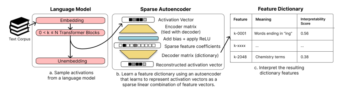
Figure 1 — Sample, train, interpret: the SAE pipeline
Figure 1 lays out this exact three-stage pipeline, sample activations, train the autoencoder, interpret the resulting dictionary, and every later experiment in this telling tests one of its three stages.
Sampling activations, training the autoencoder, reading off features concept (14 connections)
The autoencoder takes a language model's cached activation vector x and produces hidden coefficients c = ReLU(Mx + b), then reconstructs x-hat = M^T c using the same matrix M, tied between encoder and decoder. M's rows are read off afterward as the dictionary features under study. Training minimizes reconstruction error plus an L1 sparsity penalty on c (Equation 4). The method is applied mainly to residual-stream activations from the Pythia (model suite) suite: Pythia-70M (dimension 512) and Pythia-410M (dimension 1024). Because training happens after the fact on frozen, cached activations, the approach stays unsupervised and never touches the underlying language model's own weights or training.
connections
- Default (neuron/residual-stream) basis baseline — loses to → Sparse autoencoders (SAEs)
- Sparse autoencoders (SAEs) — is framed as a step toward → Enumerative safety
- Independent Component Analysis (ICA) — converges with → Sparse autoencoders (SAEs)
- Principal Component Analysis (PCA) — trails → Sparse autoencoders (SAEs)
- Sparse autoencoders (SAEs) — runs counter to the depth profile of → Residual stream hindsight
- SAE decomposition of persona vectors — applies the unsupervised machinery of → Sparse autoencoders (SAEs)
- SAE training on the MLP sublayer — stress tests → Sparse autoencoders (SAEs)
- Sharkey et al. (2023) interim research report — is validated at scale by → Sparse autoencoders (SAEs)
- Sparse dictionary learning / sparse coding — operationalized as → Sparse autoencoders (SAEs)
- Sparsity-reconstruction tradeoff (no single correct decomposition) — rules out a single canonical dictionary for → Sparse autoencoders (SAEs)
- Sparse autoencoders (SAEs) — offers an unsupervised alternative to → Steering vector hindsight
- Superposition — motivates → Sparse autoencoders (SAEs)
- Tied encoder/decoder weights — is the default configuration of → Sparse autoencoders (SAEs)
- Transformer visualization via dictionary learning (Yun et al., 2021) — is extended by → Sparse autoencoders (SAEs)
The dictionary feature as the unit of analysis concept (5 connections)
Each row of the trained matrix M is a single dictionary feature: a direction in activation space that contributes to the reconstruction whenever its coefficient is nonzero. Because the sparsity penalty forces M's rows to unit norm, a feature's row is fixed as a direction, and its activation strength alone determines how much it contributes on a given input. Every later result in the paper, interpretability scores, causal patching, and the case studies, is a claim about properties of these individual rows, not about the autoencoder as a whole.
connections
- Dictionary feature — scores unevenly across depth in → Autointerpretability score
- Dead features — hollows out the count of → Dictionary feature
- L4-norm maximization (sparse dictionary search reformulation) — predicts the heavy tailed activation of → Dictionary feature
- Monosemanticity — benchmarks → Dictionary feature
- Sparsity loss (L1 penalty on feature activations) — forces unit norm on → Dictionary feature
The sparsity penalty and its trade-off partner concept (2 connections)
The training objective (Equation 4) adds alpha times the L1 norm of c to the squared reconstruction error, penalizing how many features fire at once rather than the size of the reconstruction error directly. Alpha is the paper's central knob: raising it produces sparser, more feature-like activations at the cost of reconstruction accuracy, and its value is set separately for the residual stream (8.6e-4) and the MLP sublayer (3.2e-4), based on the active-feature sweeps in the next chapter.
connections
- Sparsity loss (L1 penalty on feature activations) — forces unit norm on → Dictionary feature
- Sparsity loss (L1 penalty on feature activations) — trades off against → Reconstruction loss
Why the encoder and decoder share weights concept (2 connections)
Tying the decoder to the encoder's transpose halves the parameter count and encodes the assumption that the direction which detects a feature and the direction that defines its effect on the reconstruction should coincide. The paper reports tied weights do not hurt performance when training on residual-stream activations, but do reduce performance on MLP activations, motivating an untied variant with separate encoder and decoder matrices used specifically for MLP-sublayer training.
connections
- Tied encoder/decoder weights — gives way to an untied variant in → SAE training on the MLP sublayer
- Tied encoder/decoder weights — is the default configuration of → Sparse autoencoders (SAEs)
Chapter 2Tuning the autoencoders before trusting the results (4 concepts)
Before the main comparisons can be trusted, the paper has to fix how large a dictionary to train, how much sparsity pressure to apply, and confirm the reconstruction is faithful enough to be worth interpreting. These sweeps, run mostly in Appendices B, C.1 and E, are not a side note: the alpha and R values fixed here are the exact ones used in every interpretability and causal-patching result that follows.
How big a dictionary: the expansion factor R concept (2 connections)
R sets the autoencoder's hidden size as dhid = R times din, controlling how overcomplete the learned dictionary is relative to the model's own activation dimension. The paper sweeps R from 0.5 (undercomplete) to 32 (far overcomplete) and finds average per-feature interpretability depends far more on layer than on R, the smallest dictionary tested scores comparably to ones dozens of times larger, while a separate quantity, the share of a layer's activation variance the dictionary explains overall, does keep rising with R. A bigger dictionary explains more of the layer without any single feature in it becoming more interpretable.
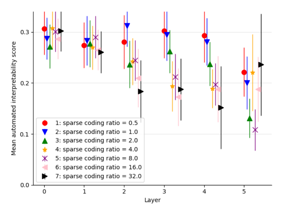
Figure 8 — Interpretability by layer across seven dictionary sizes
This is the layer-by-R sweep behind that claim: all seven ratios decline over roughly the same range across layers 0-5, about 0.27-0.31 at layer 0 down to 0.11-0.24 at layer 5, with no consistent size ranking among them.
connections
- Dictionary expansion factor (R) — governs emergence of → Dead features
- Dictionary expansion factor (R) — sets the operating point on → Sparsity-reconstruction tradeoff (no single correct decomposition)
No knee: sparsity trades smoothly against reconstruction accuracy concept (2 connections)
Sweeping alpha produces a smooth curve trading the number of simultaneously active features against unexplained reconstruction variance, with no distinct bend separating a correct operating point from an incorrect one. The paper reads this absence of a knee as weak evidence against there being one single, objectively correct sparse decomposition of a given layer's activations, a caveat that applies to every dictionary used elsewhere in the paper, since none of them is picked out as uniquely privileged by the data.
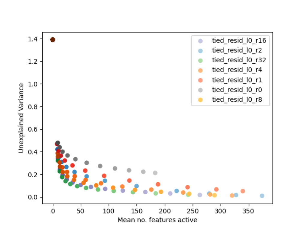
Figure 6 — Active-feature count vs. unexplained variance, by dictionary size
This MLP-layer-0 sweep across seven dictionary sizes is the source of that reading: every size traces the same knee-free curve, with one extreme point near zero active features collapsing to an unexplained variance near 1.4.
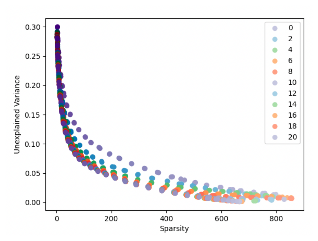
Figure 7 — Sparsity/variance tradeoff across training epochs
This companion sweep colors by training epoch instead of dictionary size, showing the tradeoff curve converges after relatively few epochs; the lowest-epoch series is visibly worse, but the rest collapse onto nearly the same curve.
connections
- Dictionary expansion factor (R) — sets the operating point on → Sparsity-reconstruction tradeoff (no single correct decomposition)
- Sparsity-reconstruction tradeoff (no single correct decomposition) — rules out a single canonical dictionary for → Sparse autoencoders (SAEs)
Feature survival: how many dictionary rows actually fire concept (2 connections)
A dictionary feature that never activates across the training corpus is dead, wasted capacity that never gets read as a feature. The paper finds residual-stream dictionaries stay almost fully alive up to roughly a 4x expansion factor before features start dropping out, which is what let it pick the alpha values used throughout, 8.6e-4 for the residual stream and 3.2e-4 for the MLP. MLP-sublayer dictionaries fare much worse: because the MLP's nonlinearity leaves large regions of input space unused, many features get stuck barely ever firing even with no sparsity penalty at all, in some cases leaving less than half a dictionary usably alive.
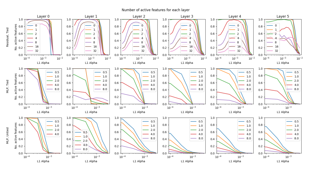
Figure 16 — Active-feature fraction vs. L1 sparsity across layers and architectures
This eighteen-panel grid is the underlying sweep: residual-stream curves (top row) stay near a fraction of 1.0 at low alpha across most ratios, while both MLP rows (tied and untied weights) start well below 1.0 even at the smallest alpha tested.
connections
- Dictionary expansion factor (R) — governs emergence of → Dead features
- Dead features — hollows out the count of → Dictionary feature
The reconstruction is never perfect concept (2 connections)
The squared-error term in Equation 4 is never driven to zero in any of the paper's trained autoencoders, meaning the dictionary always fails to capture some information present in the original activation. The paper quantifies this gap independently with a perplexity check: substituting Pythia-70M's layer-2 residual stream with its autoencoder reconstruction raises the model's perplexity on the Pile from 25 to 40, confirming that reconstruction loss reflects a real, measurable loss of information rather than a training artifact.
connections
- Reconstruction-substitution perplexity metric — independently corroborates → Reconstruction loss
- Sparsity loss (L1 penalty on feature activations) — trades off against → Reconstruction loss
Chapter 3The headline result: learned features score as more interpretable (2 concepts)
With training hyperparameters fixed, the paper turns to its central empirical claim: that individual dictionary features are more interpretable, by an automated measure, than directions found by the default neuron basis, random directions, PCA, and ICA. The comparison is run per layer of the residual stream, and the gap it finds, large in early layers, narrowing by the final layers plotted, is the result the next chapter spends four separate checks trying to break.
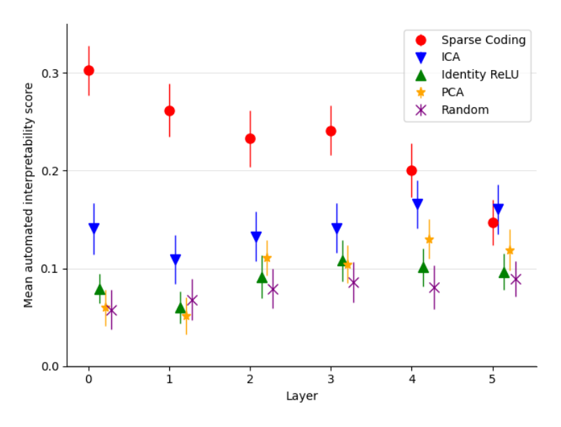
Figure 2 — Interpretability score by layer: sparse coding vs. baselines
This is the comparison itself: mean autointerpretability score across 150 features per method at each of residual-stream layers 0-5, with 95% confidence intervals. Sparse coding leads clearly at layer 0, converges toward ICA's score by layer 4, and shows minimal further gain over ICA at the final layer plotted.
How the interpretability score is computed concept (9 connections)
The score (Bills et al., 2023) is produced in three steps: sample text fragments from the first 50,000 lines of OpenWebText where a feature activates, have GPT-4 write a natural-language explanation from a handful of those fragments and their per-token activations, then have GPT-3.5 use that explanation to predict the feature's activation on held-out fragments, GPT-3.5 stands in for GPT-4 as the simulator only because its public API exposed the log-probabilities the simulation step needs. The correlation between predicted and true activations is the feature's score, so a score can run negative when the written explanation performs worse than no explanation at all.
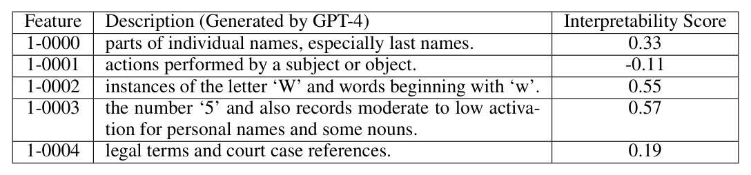
Table 1 — Layer-1 feature descriptions and interpretability scores
Table 1 previews what this pipeline outputs on five layer-1 features taken in arbitrary dictionary order: four get specific, positive-scoring descriptions (0.19 to 0.57), while one gets a vague description and a negative score of -0.11.
connections
- Dictionary feature — scores unevenly across depth in → Autointerpretability score
- GPT-3.5 — simulates activations for → Autointerpretability score
- GPT-4 — generates explanations for → Autointerpretability score
- Interpretability-vs-kurtosis/skew correlation analysis — explains variation in → Autointerpretability score
- Monosemanticity — is imperfectly proxied by → Autointerpretability score
- Autointerpretability score — prefigures the llm judge pattern of → Open-ended generation evaluation with GPT-4 rating hindsight
- Random directions baseline — anchors → Autointerpretability score
- Reconstruction-substitution perplexity metric — measures a different axis than → Autointerpretability score
- Top-and-random vs. random-only interpretability scoring — shapes fragment sampling in → Autointerpretability score
PCA as the main matrix-decomposition baseline concept (3 connections)
PCA projects the same activation dataset onto directions of maximal variance, computed with an online estimator over the same quantity of data used to train the autoencoders. It is one of four baselines run against sparse coding in the headline comparison, alongside Independent Component Analysis (ICA), the default neuron basis, and random directions, and it is the baseline the paper carries forward into the causal-patching chapter below. PCA trails sparse coding on both measures: it scores lower on autointerpretability at every layer, and later requires more patched directions and larger edit magnitudes to reach the same causal effect on the indirect-object-identification task.
connections
- Principal Component Analysis (PCA) — gets more training data than → Independent Component Analysis (ICA)
- Principal Component Analysis (PCA) — is the projection technique behind → PCA visualization of contrastive activations
- Principal Component Analysis (PCA) — trails → Sparse autoencoders (SAEs)
Chapter 4Stress-testing the interpretability advantage (4 concepts)
Because the headline gap could in principle be an artifact of an easy scoring protocol, a failure to transfer beyond the residual stream, an accident of what makes some directions heavy-tailed, or an uneven comparison between methods, the paper runs four separate checks against it. Each removes one candidate confound in turn, and each finds the same qualitative result survives, though not always at full strength.
A harsher test: scoring only on random fragments concept (3 connections)
The default scoring mixes high-activating fragments with random ones, top-and-random scoring, which could make scoring artificially easy. Rerunning with random-only scoring, fragments drawn with no regard to where a feature activates, drives every method's absolute score down, since a small random sample of a sparse feature's activations often contains no strongly-activating example at all. Sparse coding still sits clearly above all four baselines under this harsher test, especially in the earlier layers, ruling out an artifact-of-easy-scoring explanation for the headline gap.
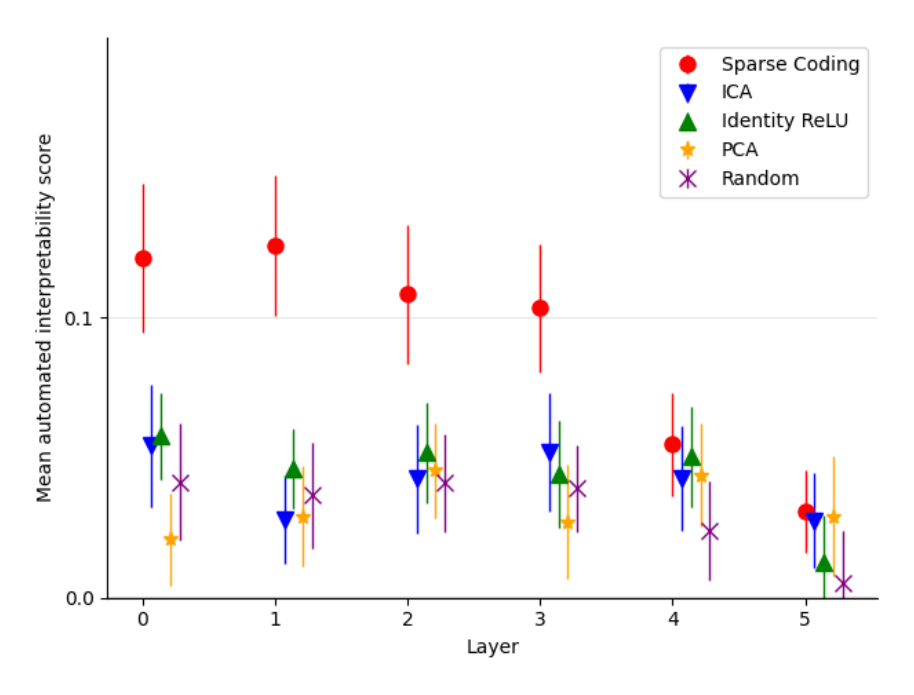
Figure 9 — Random-only interpretability scores vs. baselines by layer
This is the random-only rerun of the headline comparison: sparse coding scores roughly 0.10-0.12 in layers 0-3 against baselines clustered around 0.02-0.06, though the gap narrows at layers 4-5 as several baselines drop near zero.
connections
- Top-and-random vs. random-only interpretability scoring — shapes fragment sampling in → Autointerpretability score
- Top-and-random vs. random-only interpretability scoring — is vindicated by → Interpretability-vs-kurtosis/skew correlation analysis
- Top-K-active baseline control — tests a separate confound from → Top-and-random vs. random-only interpretability scoring
Does the advantage transfer to the MLP sublayer? concept (3 connections)
Applying the same method to MLP sublayer activations instead of the residual stream gives mixed success: many learned features are still more interpretable than individual neurons, but the large number of dead features MLP dictionaries accumulate means the living dictionary often fails to be genuinely overcomplete, and the training pipeline does not yet robustly learn overcomplete bases in the MLP's middle and later layers. Under the stricter random-only scoring, sparse coding's MLP advantage becomes inconsistent, at layer 3 it drops to about 0.03, below the Identity ReLU neuron baseline, where the residual-stream results hold up cleanly across layers.
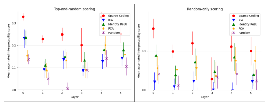
Figure 10 — MLP-layer interpretability scores vs. baselines
Both panels plot MLP layer 0-5 against interpretability score, top-and-random scoring on the left and random-only on the right: sparse coding leads clearly at layer 0, about 0.33 top-and-random, but its lead narrows and becomes uneven through the middle layers.
connections
- SAE training on the MLP sublayer — confronts → Privileged basis
- SAE training on the MLP sublayer — stress tests → Sparse autoencoders (SAEs)
- Tied encoder/decoder weights — gives way to an untied variant in → SAE training on the MLP sublayer
Why ICA is the strongest baseline concept (3 connections)
Correlating each feature's interpretability score against statistical moments of its activation distribution, pooled across all layers and five dictionary sizes, finds skew and kurtosis are the only two moments with a positive, non-negligible correlation, 0.20 and 0.15 in the table (the body text separately quotes 0.19 and 0.24), while mean and variance are essentially uncorrelated. Because ICA explicitly searches for maximally non-Gaussian, heavy-tailed directions, a search that can itself be reformulated as maximizing the L4 norm, this correlation is offered as the explanation for why ICA is consistently the strongest of the non-dictionary-learning baselines throughout the paper's comparisons.
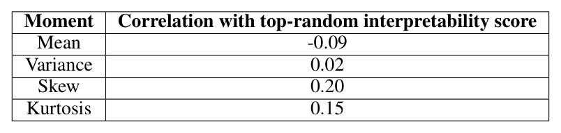
Table 2 — Interpretability correlated with activation moments
Table 2 is the correlation table itself: mean -0.09, variance 0.02, skew 0.20, kurtosis 0.15, computed over every scored residual-stream feature across all layers and expansion ratios 0.5x to 8x.
connections
- Interpretability-vs-kurtosis/skew correlation analysis — explains variation in → Autointerpretability score
- Interpretability-vs-kurtosis/skew correlation analysis — supplies empirical evidence for → Sparse dictionary learning / sparse coding
- Top-and-random vs. random-only interpretability scoring — is vindicated by → Interpretability-vs-kurtosis/skew correlation analysis
Ruling out an unfair comparison: matching active directions concept (2 connections)
A sparse dictionary feature activates on only a fraction of inputs, while a raw PCA or ICA direction is active across an entire half-space, so the interpretability gap could in principle just reflect these baselines being compared unfairly against a sparser method. The control restricts PCA and ICA to a fixed number K of simultaneously active directions per datapoint, matched to sparse coding's own average active-feature count. This adjustment does not close the gap: the Top-k variants track close to their unrestricted counterparts rather than rising toward sparse coding's score, so unequal activation density explains only a small part of the headline result.
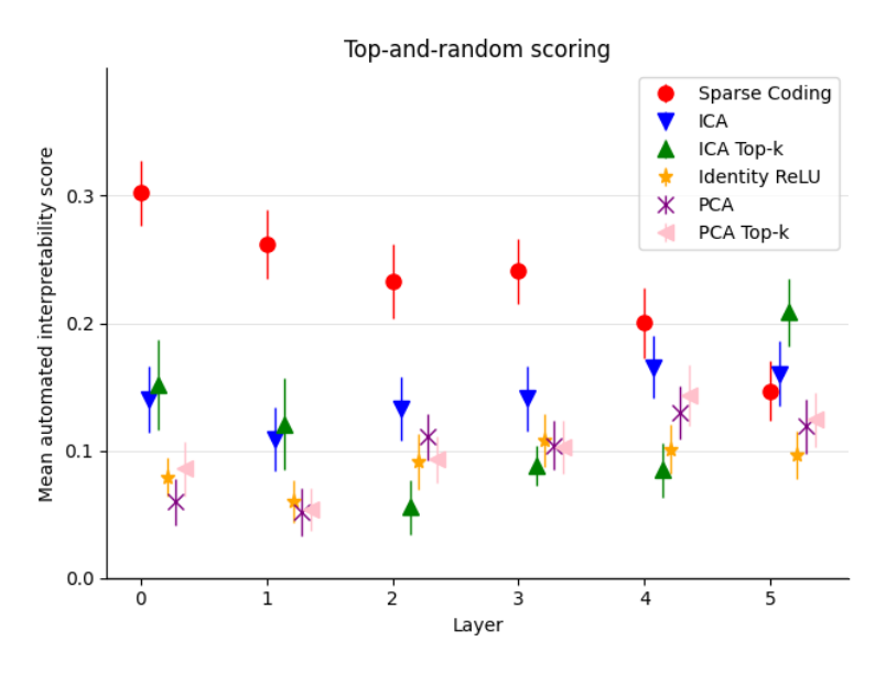
Figure 18 — Autointerpretation scores with fixed-K PCA and ICA baselines
This is the fixed-K rerun: sparse coding still leads clearly in layers 0-3, starting near 0.30 at layer 0, and ICA Top-k even scores below plain ICA at layers 2 and 3 rather than closing the gap.
connections
- Top-K-active baseline control — density matches → Independent Component Analysis (ICA)
- Top-K-active baseline control — tests a separate confound from → Top-and-random vs. random-only interpretability scoring
Chapter 5Causal evidence: patching the indirect object identification task (3 concepts)
An interpretability score only measures whether a feature's activations can be described in words; it does not show the feature actually drives the model's behavior. This chapter tests that separately with activation patching on a previously-characterized task, asking whether editing along dictionary-feature directions reproduces a target behavior with fewer, smaller edits than editing along PCA directions, and, in an appendix check, whether the result holds beyond the one layer tested in the main text.
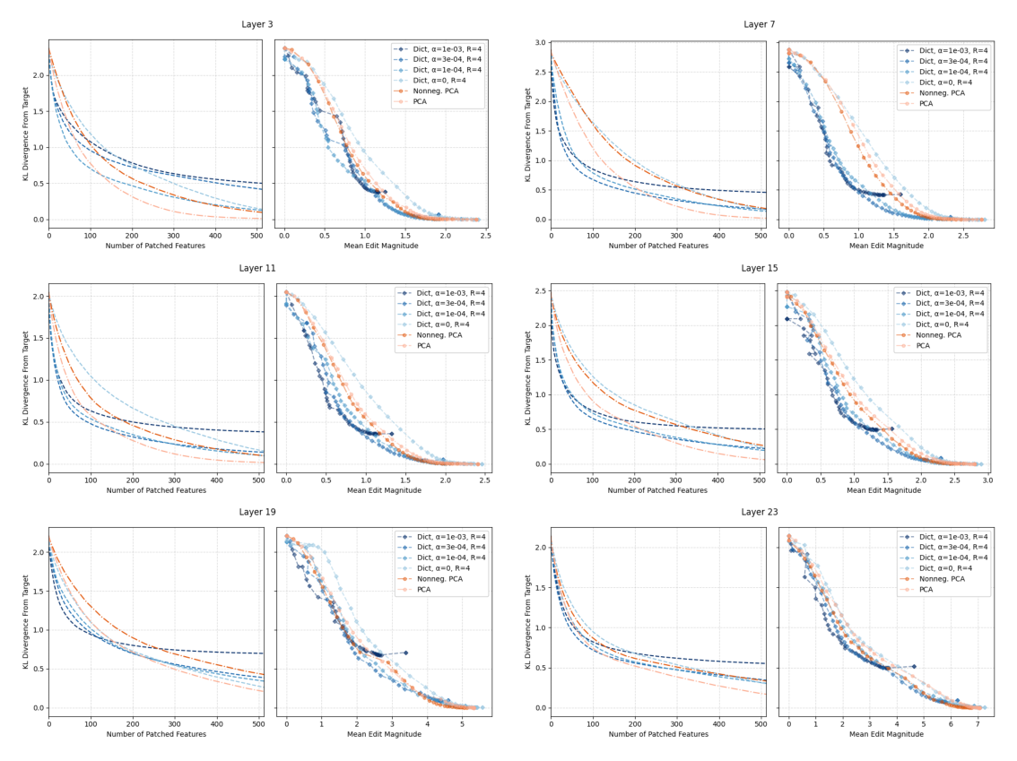
Figure 17 — IOI feature-patching precision across six more Pythia-410M layers
This appendix figure reruns the same two KL-divergence measurements across six more residual-stream layers of Pythia-410M, layers 3, 7, 11, 15, 19, 23: sparse-dictionary curves sit below and to the left of PCA's in the patched-feature-count plots at every layer tested, so the result is not specific to layer 11.
Activation patching: editing toward a counterfactual concept (1 connection)
Activation patching (Vig et al., 2020) edits a model's internal activations toward values observed on a counterfactual input and measures the resulting change in output, a way to test whether a proposed direction actually carries the causal information behind a behavior, not just a correlate of it. The paper adapts it to the Indirect Object Identification task (Wang et al., 2022), in which a model completes sentences like 'Then, Alice and Bob went to the store. Alice gave a snack to ___', chosen because the underlying mechanism was already characterized by prior work, letting the comparison isolate how precisely each decomposition's directions localize it rather than whether the mechanism exists at all.
connections
- Activation patching — is adapted into → Dictionary-feature patching procedure
Patching dictionary features versus patching PCA concept (3 connections)
The procedure, an application of activation patching to individual dictionary features, runs the model once on a counterfactual sentence to cache each feature's encoded activation, then re-runs it on the base sentence, adding the cached activation differences for a chosen feature subset into the residual stream at one layer, and measures the KL divergence between the patched output and the true counterfactual target. On layer 11 of Pythia-410M, sparse-dictionary features reach a given KL divergence with fewer patched directions and a smaller total edit magnitude than PCA components, and that advantage disappears for a non-sparse (alpha=0) dictionary, evidence that sparsity itself, not just being a learned dictionary, drives the improved localization.
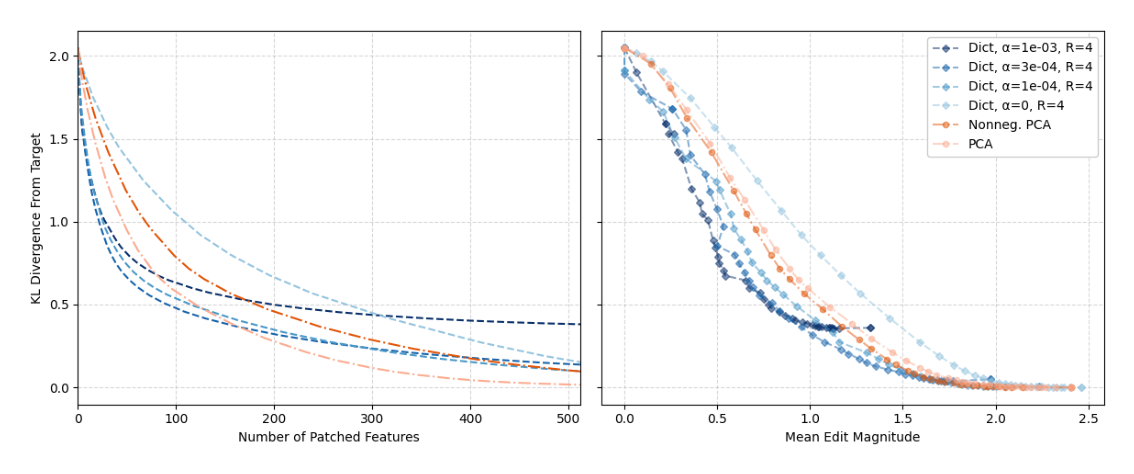
Figure 3 — IOI patching efficiency: dictionary features vs. PCA
Both panels start near a KL divergence of about 2.0 with nothing patched; the sparse-dictionary curves fall faster than PCA in the left panel, except the heaviest-sparsity dictionary (alpha=1e-3), whose curve flattens around 0.4 and never approaches zero.
connections
- Activation patching — is adapted into → Dictionary-feature patching procedure
- Dictionary-feature patching procedure — is tested against → Indirect Object Identification (IOI) task
- Less-than-rank-one ablation — edits with finer granularity than → Dictionary-feature patching procedure
Choosing which features to patch concept (1 connection)
Rather than patching an arbitrary or fixed set of directions, the paper orders candidate features by individually-estimated causal importance using the ordering procedure from Automated Circuit Discovery (Conmy et al., 2023, Algorithm 4.1), treating each feature as an independent contributor to the KL-divergence metric averaged over 50 IOI test examples. The resulting ranking, computed separately for each decomposition, dictionary features and PCA alike, is what determines the order in which directions are added along the x-axis of the patching curves, so the comparison reflects each method's most causally important directions first, not a random subset.
connections
- Automated Circuit Discovery (ACDC) — lends its ranking logic to → Automatic feature circuit detection
Chapter 6Case studies: one feature examined by hand, and one traced back (4 concepts)
Having shown that dictionary features are interpretable in aggregate and causally precise on a benchmark task, the paper closes by examining individual features directly: what text activates them, what happens to the model's output when they are ablated, and, for one feature, which earlier-layer features cause it to fire. These worked examples are where the abstract claim of monosemanticity becomes concrete.
The apostrophe feature, and its narrower relatives concept (3 connections)
Dictionary feature 556 activates almost exclusively on the apostrophe token, and using less-than-rank-one ablation, lowering the residual stream's component along the feature's direction only until the feature stops firing, to remove it from the residual stream mainly suppresses the model's predicted logit for the following 's' token, matching how apostrophes precede 's' in contractions and possessives like 'let's'. The feature does not fire on every apostrophe: two further dictionary features fire on apostrophes only in specific contraction families, one for pronoun contractions like 'I'll' and 'you'll' (ablation suppresses a broader family of endings), and one for negation contractions like 'don't' and 'won't' (ablation narrowly suppresses mainly the 't' that closes '-n't'). That the dictionary represents a single character with several distinct, narrowly-scoped features is itself evidence for fine-grained Monosemanticity.
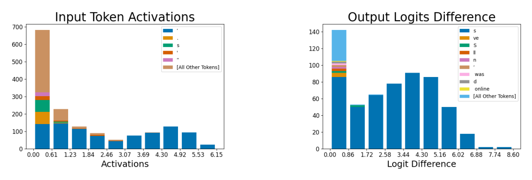
Figure 4 — Token histograms for the apostrophe feature (feature 556)
This is the core apostrophe-feature evidence: the input histogram is almost entirely apostrophe-colored from the second activation bin upward, and the output histogram shows the 's' token dominating suppressed logits, of roughly 12,000 affected in total, once ablated.
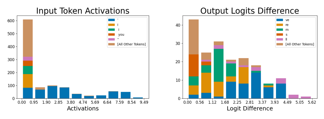
Figure 14 — Apostrophe feature for pronoun contractions ("I'll", "you'll")
This is the pronoun-contraction variant: high activations are almost solid apostrophe, with 'I' and 'you' as minor low-activation tells, and ablation suppresses a spread of endings ('ve, 're, 'm, 's, 'll) rather than one.
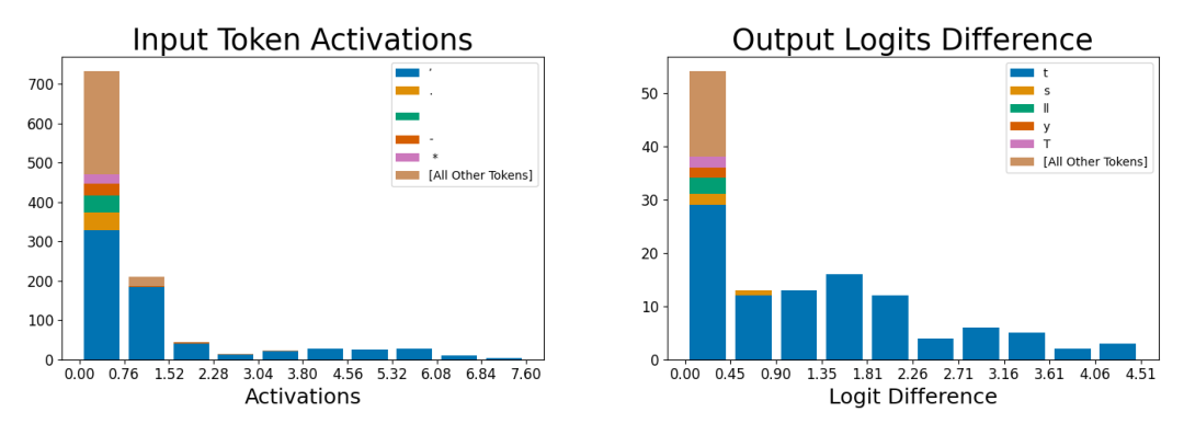
Figure 15 — Apostrophe feature for negation contractions ("don't", "won't")
This is the negation-contraction variant: ablation is far more concentrated than the pronoun variant's, with the 't' token dominating suppressed logits in nearly every bin, consistent with closing out an '-n't' contraction.
connections
- Apostrophe dictionary feature (feature 556) — divides case study labor with → Closing-parenthesis dictionary feature
- Apostrophe dictionary feature (feature 556) — is benchmarked against → Default (neuron/residual-stream) basis baseline
- Apostrophe dictionary feature (feature 556) — demonstrates the limits of → Monosemanticity
Contrast: the default-basis dimension is polysemantic concept (3 connections)
The residual stream's own coordinate basis has no particular reason to align with meaningful features, and the paper shows this concretely: the default-basis dimension that most resembles the apostrophe feature, the 10th-highest dimension the apostrophe feature itself reads from, looks like an apostrophe detector only in its highest activation bins. Across the fuller range it fires on many unrelated tokens ('and', 'one', 'part', 'number'), the textbook picture of polysemanticity, and the dimensions it draws on turn out to be outlier dimensions rather than typical basis coordinates. The clean, single-token behavior of dictionary feature 556 is therefore a property of the learned feature, not of any one default-basis direction.
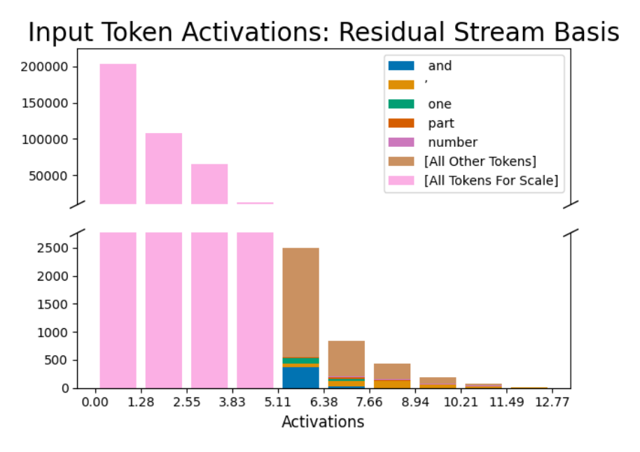
Figure 11 — Default-basis dimension resembling the apostrophe feature
The two-panel histogram makes the contrast visible only at different y-scales: the zoomed lower panel shows middle activation bins holding thousands of non-apostrophe tokens, with apostrophes becoming a large share only once total counts fall to a few hundred or fewer.
connections
- Apostrophe dictionary feature (feature 556) — is benchmarked against → Default (neuron/residual-stream) basis baseline
- Outlier dimensions — fails to elevate → Default (neuron/residual-stream) basis baseline
- Default (neuron/residual-stream) basis baseline — loses to → Sparse autoencoders (SAEs)
Monosemanticity beyond the apostrophe: code syntax and sub-word morphology concept (3 connections)
The property the case studies are built to demonstrate is monosemanticity: a feature activating for one coherent, human-interpretable pattern rather than several unrelated ones, the converse of the Polysemanticity the paper's method targets. Two further worked examples show this pattern recurs outside apostrophes: a feature that fires on the word 'if' specifically in programming contexts, whose ablation suppresses code-syntax tokens that typically follow it ('(', '&&', 'then'), and a feature that fires on the 'Dis' prefix within specific bigrams, whose ablation suppresses the word-completions that follow it ('CLAIM', 'closed', 'ordered'). In both cases the input tokens that trigger the feature and the output tokens its removal suppresses tell a matching causal story.
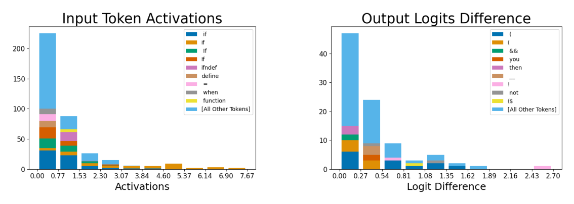
Figure 12 — 'If'-in-code feature: input and output histograms
The 'if' feature's input tokens are several tokenizations of 'if' plus code-specific tokens ('ifndef', 'define', 'when'); its output panel shows ablation most suppresses '(', '&&', 'then', and '!', tokens that typically follow 'if' in code.
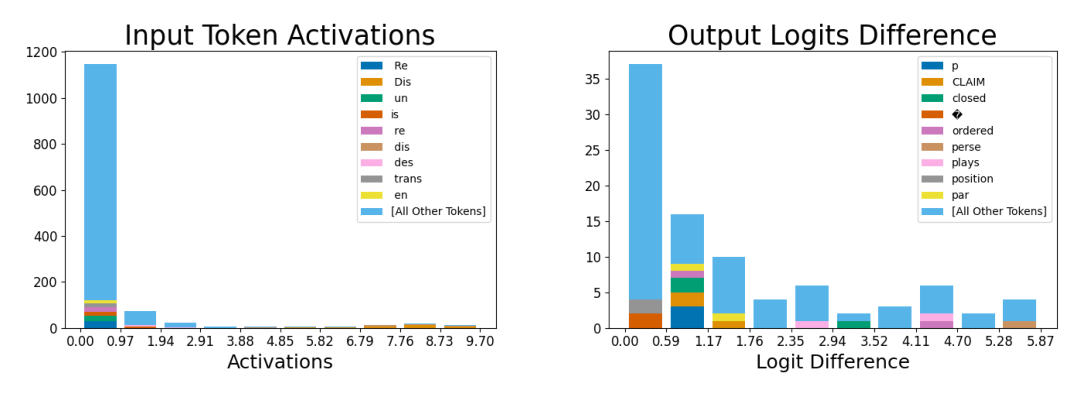
Figure 13 — 'Dis'-prefix feature: input and output histograms
The 'Dis'-prefix feature's highest-activation bins are almost entirely prefix fragments ('Dis', 're', 'un', 'trans'); ablation most suppresses specific word-completions like 'CLAIM', 'closed', and 'ordered' that follow the prefix.
connections
- Apostrophe dictionary feature (feature 556) — demonstrates the limits of → Monosemanticity
- Monosemanticity — is imperfectly proxied by → Autointerpretability score
- Monosemanticity — benchmarks → Dictionary feature
Tracing a feature back through the layers that cause it concept (4 connections)
Beyond a single feature's inputs and outputs, the paper traces causal dependencies across layers: given a target feature, sample contexts where it strongly activates, then for each feature in the previous layer, ablate it and measure how much the target's activation drops, ranking previous-layer features by that effect and optionally recursing. Applied to the layer-5 closing-parenthesis feature, whose unembedding directly predicts closing-parenthesis tokens, this produces a multi-layer causal tree with two branches feeding the root, one tracking generic parenthetical context, one tracking acronyms specifically, that merge just before the final feature. The paper contrasts this success with a weight-based alternative tried between layers 4 and 5, multiplying a feature through the MLP weights and checking cosine similarity, which found no meaningful connections, likely because the resulting vector left the model's typical activation distribution.
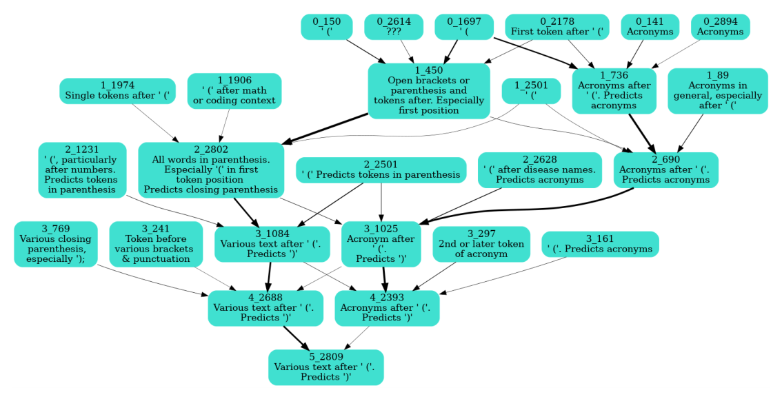
Figure 5 — Causal-tree circuit for the closing-parenthesis feature
This is the causal tree itself: arrow thickness encodes how much a downstream feature's activation dropped when its upstream candidate was ablated, so the thickest paths are the dominant causes feeding the closing-parenthesis feature.
connections
- Automated Circuit Discovery (ACDC) — lends its ranking logic to → Automatic feature circuit detection
- Closing-parenthesis dictionary feature — seeds → Automatic feature circuit detection
- Automatic feature circuit detection — is offered as a concrete step toward → Enumerative safety
- Weight-based feature connection attempt (failed method) — is the failed precursor to → Automatic feature circuit detection
The corpus's first paper that reads a model's internals without trying to change its behavior: everything on its introduced shelf is instrument-making. The sparse autoencoder itself arrives with its dictionary features, the ℓ1 sparsity penalty and reconstruction loss whose tradeoff the paper concedes has no single correct answer, the tied weights and expansion factor that fix its shape, and the dead features that appear as dictionaries grow; the proof side adds feature patching with finer-than-rank-one ablations, automatic feature circuits — with the failed weight-based route honestly recorded — and the apostrophe and closing-parenthesis case studies. The refined shelf holds a single concept, and the choice is telling: the residual stream, the steering papers' injection site, becomes the object under the microscope, its mostly-unprivileged basis and outlier dimensions examined rather than assumed. The inherited shelf — 25 of 44 concepts — is the problem and the judging apparatus: the Polysemanticity and Superposition diagnosis it answers, the sparse-coding lineage it scales through Yun et al. and Sharkey et al., the autointerpretability protocol and GPT-4 that grade its features, Activation patching and the IOI task that test them, the PCA, ICA, and default-basis ladder it must beat, the Pythia-on-Pile testbed that scopes its claims, and the enumerative safety ambition that gives the exercise its safety meaning — an ambition the 2025 paper already cashes a first check on, running these autoencoders over its own persona vectors.
Read at
Introduced here introduced (18 concepts, in reading order)
Dictionary expansion factor (R) (2 connections) §“2 TAKING FEATURES OUT OF SUPERPOSITION WITH SPARSE DICTIONARY LEARNING”, p. 2
- Dictionary expansion factor (R) — governs emergence of → Dead features
- Dictionary expansion factor (R) — sets the operating point on → Sparsity-reconstruction tradeoff (no single correct decomposition)
The hyperparameter R controlling the ratio of the autoencoder's hidden dimension to the model's activation dimension (dhid = R x din), governing how overcomplete the learned feature dictionary is. The paper sweeps R and finds interpretability gains hold even for undercomplete dictionaries (R<1), with larger dictionaries explaining more of the overall activation variance.Dictionary feature (5 connections) §“2 TAKING FEATURES OUT OF SUPERPOSITION WITH SPARSE DICTIONARY LEARNING”, p. 2
- Dictionary feature — scores unevenly across depth in → Autointerpretability score
- Dead features — hollows out the count of → Dictionary feature
- L4-norm maximization (sparse dictionary search reformulation) — predicts the heavy tailed activation of → Dictionary feature
- Monosemanticity — benchmarks → Dictionary feature
- Sparsity loss (L1 penalty on feature activations) — forces unit norm on → Dictionary feature
A single learned row of the sparse autoencoder's weight matrix M (equivalently, one hidden unit of the autoencoder), representing a direction in activation space used to reconstruct inputs as a sparse linear combination. Individual dictionary features are the paper's central unit of analysis, examined for interpretability (Section 3), causal importance (Section 4), and monosemanticity (Section 5).Sparse autoencoders (SAEs) (14 connections) §“2 TAKING FEATURES OUT OF SUPERPOSITION WITH SPARSE DICTIONARY LEARNING”, p. 2
- Default (neuron/residual-stream) basis baseline — loses to → Sparse autoencoders (SAEs)
- Sparse autoencoders (SAEs) — is framed as a step toward → Enumerative safety
- Independent Component Analysis (ICA) — converges with → Sparse autoencoders (SAEs)
- Principal Component Analysis (PCA) — trails → Sparse autoencoders (SAEs)
- Sparse autoencoders (SAEs) — runs counter to the depth profile of → Residual stream hindsight
- SAE decomposition of persona vectors — applies the unsupervised machinery of → Sparse autoencoders (SAEs)
- SAE training on the MLP sublayer — stress tests → Sparse autoencoders (SAEs)
- Sharkey et al. (2023) interim research report — is validated at scale by → Sparse autoencoders (SAEs)
- Sparse dictionary learning / sparse coding — operationalized as → Sparse autoencoders (SAEs)
- Sparsity-reconstruction tradeoff (no single correct decomposition) — rules out a single canonical dictionary for → Sparse autoencoders (SAEs)
- Sparse autoencoders (SAEs) — offers an unsupervised alternative to → Steering vector hindsight
- Superposition — motivates → Sparse autoencoders (SAEs)
- Tied encoder/decoder weights — is the default configuration of → Sparse autoencoders (SAEs)
- Transformer visualization via dictionary learning (Yun et al., 2021) — is extended by → Sparse autoencoders (SAEs)
This paper trains single-hidden-layer, ReLU, tied-weight autoencoders with an L1 sparsity penalty on their hidden activations to decompose language model activations into an overcomplete, sparsely-activating dictionary of features. It is one of the two founding empirical demonstrations (alongside the concurrent Anthropic 'Towards Monosemanticity' work) that this architecture recovers features that are more interpretable, more monosemantic, and more causally precise than PCA/ICA/neuron-basis baselines, establishing SAEs as a scalable method for resolving superposition.Tied encoder/decoder weights (2 connections) §“2 TAKING FEATURES OUT OF SUPERPOSITION WITH SPARSE DICTIONARY LEARNING”, p. 2
- Tied encoder/decoder weights — gives way to an untied variant in → SAE training on the MLP sublayer
- Tied encoder/decoder weights — is the default configuration of → Sparse autoencoders (SAEs)
The design choice of using a single weight matrix (transposed between encoder and decoder) for the SAE, adopted because it encodes the expectation that a feature's detecting and defining directions coincide, halves memory cost, and removes encoder/decoder direction ambiguity. The paper finds tied weights hurt performance on MLP activations, motivating an untied variant with separate encoder/decoder matrices for that setting.Reconstruction loss (2 connections) §“2 TAKING FEATURES OUT OF SUPERPOSITION WITH SPARSE DICTIONARY LEARNING”, p. 3
- Reconstruction-substitution perplexity metric — independently corroborates → Reconstruction loss
- Sparsity loss (L1 penalty on feature activations) — trades off against → Reconstruction loss
The ||x - x-hat||^2 term in the SAE training objective (Equation 4), the standard squared-error measure of how well the reconstructed activation vector matches the original. The paper notes this loss is never driven to zero, showing the dictionary fails to capture all information in a layer's activations, a gap it also quantifies via the reconstruction-perplexity metric.Sparsity loss (L1 penalty on feature activations) (2 connections) §“2 TAKING FEATURES OUT OF SUPERPOSITION WITH SPARSE DICTIONARY LEARNING”, p. 3
- Sparsity loss (L1 penalty on feature activations) — forces unit norm on → Dictionary feature
- Sparsity loss (L1 penalty on feature activations) — trades off against → Reconstruction loss
The alpha*||c||_1 term in the autoencoder's training objective (Equation 4), penalizing the L1 norm of the hidden-layer coefficients c to encourage sparse feature activations. The sparsity coefficient alpha is the paper's key hyperparameter, swept throughout to trade off sparsity against reconstruction accuracy.Dictionary-feature patching procedure (3 connections) §“4.1 ADAPTING ACTIVATION PATCHING TO DICTIONARY FEATURES”, p. 6
- Activation patching — is adapted into → Dictionary-feature patching procedure
- Dictionary-feature patching procedure — is tested against → Indirect Object Identification (IOI) task
- Less-than-rank-one ablation — edits with finer granularity than → Dictionary-feature patching procedure
The paper's specific patching procedure for dictionary features: run the model on a counterfactual sentence, cache the encoded feature activations, then re-run on the base sentence and add the encoded activation differences for a chosen feature subset F into the residual stream, measuring KL divergence between patched and target output logits. Found to reach a given KL divergence with fewer patched features and smaller edit magnitude than patching an equivalent number of PCA components.Apostrophe dictionary feature (feature 556) (3 connections) §“5.1 INPUT: DICTIONARY FEATURES ARE HIGHLY MONOSEMANTIC”, p. 7
- Apostrophe dictionary feature (feature 556) — divides case study labor with → Closing-parenthesis dictionary feature
- Apostrophe dictionary feature (feature 556) — is benchmarked against → Default (neuron/residual-stream) basis baseline
- Apostrophe dictionary feature (feature 556) — demonstrates the limits of → Monosemanticity
A case-study dictionary feature that activates almost exclusively on apostrophe tokens, the paper's central worked example of monosemanticity. Ablating it specifically suppresses the logit for the following 's' token, illustrating that dictionary features have intuitive, predictable causal effects on model outputs, in contrast to the corresponding polysemantic default-basis dimension.Less-than-rank-one ablation (1 connection) §“5.2 OUTPUT: DICTIONARY FEATURES HAVE INTUITIVE EFFECTS ON THE LOGITS”, p. 7
- Less-than-rank-one ablation — edits with finer granularity than → Dictionary-feature patching procedure
A specific ablation technique that lowers a residual-stream activation's component along a feature's direction only up to the point where that feature is no longer active, rather than a full-magnitude subtraction. Used to measure a dictionary feature's causal effect on next-token logits in the apostrophe-feature case study.Automatic feature circuit detection (4 connections) §“5.3 INTERMEDIATE FEATURES: DICTIONARY FEATURES ALLOW AUTOMATIC CIRCUIT DETECTION”, p. 8
- Automated Circuit Discovery (ACDC) — lends its ranking logic to → Automatic feature circuit detection
- Closing-parenthesis dictionary feature — seeds → Automatic feature circuit detection
- Automatic feature circuit detection — is offered as a concrete step toward → Enumerative safety
- Weight-based feature connection attempt (failed method) — is the failed precursor to → Automatic feature circuit detection
A method for tracing causal dependencies between dictionary features in adjacent layers: given a target feature, sample contexts where it strongly activates, then ablate each previous-layer feature and rank features by how much their ablation decreases the target's activation, optionally recursing to build a multi-layer causal tree. Demonstrated on a layer-5 feature that predicts closing parentheses, yielding an interpretable circuit of upstream features.Closing-parenthesis dictionary feature (2 connections) §“5.3 INTERMEDIATE FEATURES: DICTIONARY FEATURES ALLOW AUTOMATIC CIRCUIT DETECTION”, p. 8
- Apostrophe dictionary feature (feature 556) — divides case study labor with → Closing-parenthesis dictionary feature
- Closing-parenthesis dictionary feature — seeds → Automatic feature circuit detection
A case-study dictionary feature in layer 5 whose unembedding directly predicts closing-parenthesis tokens, used to illustrate the paper's feature-circuit-detection method by tracing which upstream features (detecting dates, acronyms, and other parenthesis-preceding phrases) cause it to activate.Reconstruction-substitution perplexity metric (2 connections) §“6.2 LIMITATIONS AND FUTURE WORK”, p. 9
- Reconstruction-substitution perplexity metric — measures a different axis than → Autointerpretability score
- Reconstruction-substitution perplexity metric — independently corroborates → Reconstruction loss
A fidelity check in which a layer's activations are replaced with the SAE's reconstruction of them and the resulting increase in the model's perplexity on the Pile is measured, quantifying information lost by the dictionary. Reported as rising from 25 to 40 when substituting Pythia-70M's layer-2 residual stream with its reconstruction, evidencing that reconstruction loss is not yet near zero.Sparsity-reconstruction tradeoff (no single correct decomposition) (2 connections) §“B SPARSE AUTOENCODER TRAINING AND HYPERPARAMETER SELECTION”, p. 12
- Dictionary expansion factor (R) — sets the operating point on → Sparsity-reconstruction tradeoff (no single correct decomposition)
- Sparsity-reconstruction tradeoff (no single correct decomposition) — rules out a single canonical dictionary for → Sparse autoencoders (SAEs)
The paper's empirical finding, from sweeping the sparsity coefficient alpha, that there is a smooth tradeoff between the number of active features and unexplained reconstruction variance, with no distinct 'knee' or single best operating point. Taken as weak evidence against there being one uniquely correct sparse decomposition of a given activation space.Dead features (2 connections) §“C.3 INTERPRETING THE MLP SUBLAYER”, p. 15
- Dictionary expansion factor (R) — governs emergence of → Dead features
- Dead features — hollows out the count of → Dictionary feature
Dictionary features that never activate across the training corpus, wasting dictionary capacity. The paper finds residual-stream dictionaries stay overcomplete (few dead features) up to roughly a 4x expansion factor, while MLP-sublayer dictionaries suffer many dead features even without a sparsity penalty, in some cases leaving less than half the dictionary usably 'alive'.Interpretability-vs-kurtosis/skew correlation analysis (3 connections) §“C.4 INTERPRETABILITY SCORES CORRELATE WITH KURTOSIS AND SKEW OF ACTIVATION”, p. 15
- Interpretability-vs-kurtosis/skew correlation analysis — explains variation in → Autointerpretability score
- Interpretability-vs-kurtosis/skew correlation analysis — supplies empirical evidence for → Sparse dictionary learning / sparse coding
- Top-and-random vs. random-only interpretability scoring — is vindicated by → Interpretability-vs-kurtosis/skew correlation analysis
An analysis correlating a dictionary feature's autointerpretability score with statistical moments of its activation distribution, finding weak positive correlations (0.19-0.24) with skew and kurtosis respectively. Used to argue that more heavy-tailed features are more interpretable, and to explain why ICA -- which explicitly maximizes non-Gaussianity -- is the strongest of the non-SAE baselines.SAE training on the MLP sublayer (3 connections) §“C.3 INTERPRETING THE MLP SUBLAYER”, p. 15
- SAE training on the MLP sublayer — confronts → Privileged basis
- SAE training on the MLP sublayer — stress tests → Sparse autoencoders (SAEs)
- Tied encoder/decoder weights — gives way to an untied variant in → SAE training on the MLP sublayer
An extension of the paper's method to train dictionaries on MLP sublayer activations rather than the residual stream, finding 'mixed success': many features are more interpretable than individual neurons, but the approach suffers from large numbers of dead features and does not yet robustly learn overcomplete bases in intermediate or later MLP layers.Weight-based feature connection attempt (failed method) (1 connection) §“D.4 FAILED INTERPRETABILITY METHODS”, p. 17
- Weight-based feature connection attempt (failed method) — is the failed precursor to → Automatic feature circuit detection
A failed alternative method for connecting features across layers, tried by multiplying a layer-4 feature through the MLP weights and checking cosine similarity with layer-5 features. It found no meaningful connections, likely because the resulting vector went out-of-distribution; reported as a negative result contrasting with the ablation-based feature-circuit-detection method that did succeed.Top-K-active baseline control (2 connections) §“G TOP K COMPARISONS”, p. 18
- Top-K-active baseline control — density matches → Independent Component Analysis (ICA)
- Top-K-active baseline control — tests a separate confound from → Top-and-random vs. random-only interpretability scoring
A control experiment (Appendix G) restricting the PCA and ICA baselines to a fixed number K of simultaneously 'active' directions per datapoint, matched to the SAE's average active-feature count, to test whether SAE's interpretability advantage merely reflects its lower per-datapoint activation density rather than genuinely better features. Finds this adjustment explains only a small fraction of the interpretability gap.
Refined here refined (1 concept, in reading order)
Residual stream (6 connections) §“2 TAKING FEATURES OUT OF SUPERPOSITION WITH SPARSE DICTIONARY LEARNING”, p. 2
- Behavioral clustering — localizes suddenly in → Residual stream
- Residual stream — is the injection site whose growth constrains → Contrastive Activation Addition (CAA)
- Privileged basis — is absent from → Residual stream
- Response-conditioned contrastive vector computation — sweeps and selects a layer within → Residual stream
- Sparse autoencoders (SAEs) — runs counter to the depth profile of → Residual stream hindsight
- Steering outside the residual stream (proposed extension) — would localize representations beyond → Residual stream
The transformer's running sum of layer outputs, this paper's primary object of study: sparse autoencoders are trained mainly on residual-stream activations, and the paper investigates whether the residual stream has a 'privileged basis' and how outlier dimensions relate to interpretable dictionary features.
Inherited — used, not invented here inherited (25 concepts, in reading order)
Mechanistic interpretability (2 connections) §“1 INTRODUCTION”, p. 1
- Mechanistic interpretability — is the field that dreams of → Enumerative safety
- Polysemanticity — blocks → Mechanistic interpretability
A research agenda that seeks to understand neural networks by reverse-engineering their internal computations into human-understandable parts, aiming to enable verification, targeted editing, and mitigation of risks such as deceptive behavior. Named in the introduction as the field this paper's sparse-autoencoder method aims to advance, offering it as 'a foundation for future mechanistic interpretability work.'Polysemanticity (2 connections) §“1 INTRODUCTION”, p. 1
- Polysemanticity — blocks → Mechanistic interpretability
- Superposition — manifests as → Polysemanticity
The phenomenon in which individual neurons (or other analysis units) activate in multiple, semantically unrelated contexts, preventing concise human-understandable explanations of a network's internal computation. Named as the paper's central roadblock in the abstract; the paper's entire method is aimed at finding a decomposition of activation space with reduced polysemanticity.Superposition (2 connections) §“1 INTRODUCTION”, p. 1
- Superposition — manifests as → Polysemanticity
- Superposition — motivates → Sparse autoencoders (SAEs)
A hypothesized cause of polysemanticity (Elhage et al., 2022b) in which a network represents more features than it has dimensions by assigning them to an overcomplete set of non-orthogonal directions, relying on activation sparsity to limit interference. The paper's stated goal is to resolve superposition in language models by recovering these directions via sparse dictionary learning.- Pythia (model suite) §“2 TAKING FEATURES OUT OF SUPERPOSITION WITH SPARSE DICTIONARY LEARNING”, p. 2A suite of open, reproducible language models of varying sizes (Biderman et al., 2023). This paper trains sparse autoencoders on the residual streams of Pythia-70M (din=512) and Pythia-410M (din=1024), its primary experimental subjects throughout.
Sharkey et al. (2023) interim research report (1 connection) §“1 INTRODUCTION”, p. 2
- Sharkey et al. (2023) interim research report — is validated at scale by → Sparse autoencoders (SAEs)
An unpublished interim research report ('Taking features out of superposition with sparse autoencoders,' Sharkey, Braun & Millidge, 2023) that first proposed training sparse autoencoders on language model activations to address superposition. Cited as the direct motivation and foundation this paper builds on and scales up.Sparse dictionary learning / sparse coding (3 connections) §“2 TAKING FEATURES OUT OF SUPERPOSITION WITH SPARSE DICTIONARY LEARNING”, p. 2
- Interpretability-vs-kurtosis/skew correlation analysis — supplies empirical evidence for → Sparse dictionary learning / sparse coding
- L4-norm maximization (sparse dictionary search reformulation) — reformulates → Sparse dictionary learning / sparse coding
- Sparse dictionary learning / sparse coding — operationalized as → Sparse autoencoders (SAEs)
A prior mathematical framework (Olshausen & Field, 1997; Lee et al., 2006), originally developed to model sparse coding in the visual cortex, for expressing data as sparse linear combinations of an overcomplete set of learned basis vectors (a 'dictionary'). This paper's sparse autoencoder is presented as a scalable neural-network implementation of this framework applied to language model activations.Transformer visualization via dictionary learning (Yun et al., 2021) (1 connection) §“1 INTRODUCTION”, p. 2
- Transformer visualization via dictionary learning (Yun et al., 2021) — is extended by → Sparse autoencoders (SAEs)
Prior work applying sparse dictionary learning to residual stream activations across all layers of a language model simultaneously, framing token representations as a linear superposition of transformer factors. Cited as closely related prior work alongside Sharkey et al. (2023), applying a similar technique but without the interpretability and causal-localization evaluations this paper contributes.Autointerpretability score (9 connections) §“3.1 INTERPRETABILITY AT SCALE”, p. 3
- Dictionary feature — scores unevenly across depth in → Autointerpretability score
- GPT-3.5 — simulates activations for → Autointerpretability score
- GPT-4 — generates explanations for → Autointerpretability score
- Interpretability-vs-kurtosis/skew correlation analysis — explains variation in → Autointerpretability score
- Monosemanticity — is imperfectly proxied by → Autointerpretability score
- Autointerpretability score — prefigures the llm judge pattern of → Open-ended generation evaluation with GPT-4 rating hindsight
- Random directions baseline — anchors → Autointerpretability score
- Reconstruction-substitution perplexity metric — measures a different axis than → Autointerpretability score
- Top-and-random vs. random-only interpretability scoring — shapes fragment sampling in → Autointerpretability score
An automated interpretability metric (Bills et al., 2023) in which a language model is shown text where a feature activates, writes a natural-language explanation of the feature, and then a (possibly different) language model uses that explanation to predict the feature's activations on held-out text; the correlation between predicted and actual activations is the score. This paper applies it at scale (GPT-4 generates explanations, GPT-3.5 simulates activations) as its primary measure of dictionary-feature interpretability, run across thousands of features and several baselines.Default (neuron/residual-stream) basis baseline (3 connections) §“3.2 SPARSE DICTIONARY FEATURES ARE MORE INTERPRETABLE THAN BASELINES”, p. 3
- Apostrophe dictionary feature (feature 556) — is benchmarked against → Default (neuron/residual-stream) basis baseline
- Outlier dimensions — fails to elevate → Default (neuron/residual-stream) basis baseline
- Default (neuron/residual-stream) basis baseline — loses to → Sparse autoencoders (SAEs)
Treating individual neurons, or for the residual stream individual basis coordinates, as the units of analysis, used as a naive baseline against which the paper's dictionary features are compared for autointerpretability. The residual-stream default basis is shown, via the apostrophe-dimension case study, to be polysemantic where the corresponding dictionary feature is monosemantic.Independent Component Analysis (ICA) (3 connections) §“3.2 SPARSE DICTIONARY FEATURES ARE MORE INTERPRETABLE THAN BASELINES”, p. 3
- Principal Component Analysis (PCA) — gets more training data than → Independent Component Analysis (ICA)
- Independent Component Analysis (ICA) — converges with → Sparse autoencoders (SAEs)
- Top-K-active baseline control — density matches → Independent Component Analysis (ICA)
A standard technique that finds maximally non-Gaussian (statistically independent) directions in data, used as a baseline decomposition of model activations. ICA is consistently the strongest of the non-dictionary-learning baselines, which the paper attributes to interpretability correlating with activation kurtosis and skew -- properties ICA directly optimizes for.Principal Component Analysis (PCA) (3 connections) §“3.2 SPARSE DICTIONARY FEATURES ARE MORE INTERPRETABLE THAN BASELINES”, p. 3
- Principal Component Analysis (PCA) — gets more training data than → Independent Component Analysis (ICA)
- Principal Component Analysis (PCA) — is the projection technique behind → PCA visualization of contrastive activations
- Principal Component Analysis (PCA) — trails → Sparse autoencoders (SAEs)
Used here as one of four baseline decompositions of language model activations (alongside the default basis, random directions, and ICA), against which the paper's sparse dictionary features are compared both for autointerpretability score and for IOI-patching precision, underperforming the learned dictionaries in both cases.Random directions baseline (1 connection) §“3.2 SPARSE DICTIONARY FEATURES ARE MORE INTERPRETABLE THAN BASELINES”, p. 3
- Random directions baseline — anchors → Autointerpretability score
Randomly sampled directions in activation space, used as a lower-bound baseline for autointerpretability comparisons alongside the default basis, PCA, and ICA.Activation patching (1 connection) §“4 IDENTIFYING CAUSALLY-IMPORTANT DICTIONARY FEATURES FOR INDIRECT OBJECT IDENTIFICATION”, p. 5
- Activation patching — is adapted into → Dictionary-feature patching procedure
A causal mediation analysis technique (Vig et al., 2020) in which a model's internal activations are edited toward values observed on a counterfactual input and the resulting change in output is measured. This paper adapts it to dictionary features -- patching feature-encoded activation differences into the residual stream and measuring KL divergence from a target output -- to test how precisely SAE features localize the Indirect Object Identification behavior, compared to patching PCA components.Indirect Object Identification (IOI) task (1 connection) §“4 IDENTIFYING CAUSALLY-IMPORTANT DICTIONARY FEATURES FOR INDIRECT OBJECT IDENTIFICATION”, p. 5
- Dictionary-feature patching procedure — is tested against → Indirect Object Identification (IOI) task
A previously-studied model behavior (Wang et al., 2022) in which a language model completes sentences such as 'Alice and Bob went to the store. Alice gave a snack to ___' by correctly naming the indirect object. Used as this paper's case-study task for testing how precisely dictionary features localize a known circuit, via activation patching and KL-divergence comparisons against PCA.Automated Circuit Discovery (ACDC) (1 connection) §“4.1 ADAPTING ACTIVATION PATCHING TO DICTIONARY FEATURES”, p. 6
- Automated Circuit Discovery (ACDC) — lends its ranking logic to → Automatic feature circuit detection
A prior algorithm (Conmy et al., 2023) for automatically discovering the subgraph of a network responsible for a behavior. This paper reuses ACDC's ordering procedure (its Algorithm 4.1) to rank dictionary features by their individual causal contribution to reducing KL divergence on the IOI task, producing the feature subset used in the dictionary-feature-patching experiments.Monosemanticity (3 connections) §“5.1 INPUT: DICTIONARY FEATURES ARE HIGHLY MONOSEMANTIC”, p. 7
- Apostrophe dictionary feature (feature 556) — demonstrates the limits of → Monosemanticity
- Monosemanticity — is imperfectly proxied by → Autointerpretability score
- Monosemanticity — benchmarks → Dictionary feature
The property of a feature or direction activating for a single, coherent, human-interpretable concept -- the converse of polysemanticity. The paper's case studies (the apostrophe and closing-parenthesis features) are framed as demonstrating that learned dictionary features are highly monosemantic compared to neurons or other baseline directions.Enumerative safety (3 connections) §“6.3 CONCLUSION”, p. 9
- Automatic feature circuit detection — is offered as a concrete step toward → Enumerative safety
- Mechanistic interpretability — is the field that dreams of → Enumerative safety
- Sparse autoencoders (SAEs) — is framed as a step toward → Enumerative safety
An aspirational goal in interpretability research (Elhage et al., 2022b) of producing a complete, human-understandable enumeration of a model's features sufficient to guarantee it will not perform dangerous behaviors such as deception. Invoked in the paper's conclusion as the long-term motivation its sparse-autoencoder method is framed as a step toward.GPT-3.5 (1 connection) §“A AUTOINTERPRETATION PROTOCOL”, p. 11
- GPT-3.5 — simulates activations for → Autointerpretability score
OpenAI's GPT-3.5 model, used as the 'simulator' in the autointerpretability pipeline: given a feature's GPT-4-written explanation, it predicts the feature's per-token activations on held-out text, which are then correlated with ground truth to produce the interpretability score. Substituted for GPT-4 (used for simulation in the original Bills et al. protocol) because OpenAI's public GPT-3.5 API exposed the logprobs the simulation step requires, while its GPT-4 API did not at the time.GPT-4 (3 connections) §“A AUTOINTERPRETATION PROTOCOL”, p. 11
- GPT-4 — generates explanations for → Autointerpretability score
- GPT-4 — authors → Custom refusal contrastive dataset
- GPT-4 — rates outputs for → Open-ended generation evaluation with GPT-4 rating
OpenAI's large language model, used in this paper as the explainer model in the autointerpretability pipeline: given highly-activating text fragments and per-token activations, GPT-4 generates a natural-language description of what a dictionary feature detects.- OpenWebText §“A AUTOINTERPRETATION PROTOCOL”, p. 11A public web-text dataset used as the source of text fragments (the first 50,000 lines) on which dictionary feature activations are sampled for the autointerpretability protocol.
- The Pile §“B SPARSE AUTOENCODER TRAINING AND HYPERPARAMETER SELECTION”, p. 12A large public webtext corpus (Gao et al., 2020) used to generate the activation datasets the sparse autoencoders are trained on, and to measure perplexity when testing how much information is lost by reconstructing a layer's activations from its dictionary features.
Top-and-random vs. random-only interpretability scoring (3 connections) §“C.2 HIGH INTERPRETABILITY SCORES ARE NOT AN ARTEFACT OF TOP SCORING”, p. 13
- Top-and-random vs. random-only interpretability scoring — shapes fragment sampling in → Autointerpretability score
- Top-and-random vs. random-only interpretability scoring — is vindicated by → Interpretability-vs-kurtosis/skew correlation analysis
- Top-K-active baseline control — tests a separate confound from → Top-and-random vs. random-only interpretability scoring
A distinction, from the Bills et al. (2023) protocol, in how text fragments are chosen when scoring an autointerpretability explanation: 'top-and-random' scoring mixes highly-activating fragments with randomly sampled ones (the paper's default), while the stricter 'random-only' scoring uses only random fragments. The paper reruns its comparison using random-only scoring (Appendix C.2) and finds its learned features still outperform baselines, ruling out an artifact-of-top-scoring explanation for its results.L4-norm maximization (sparse dictionary search reformulation) (2 connections) §“C.4 INTERPRETABILITY SCORES CORRELATE WITH KURTOSIS AND SKEW OF ACTIVATION”, p. 15
- L4-norm maximization (sparse dictionary search reformulation) — predicts the heavy tailed activation of → Dictionary feature
- L4-norm maximization (sparse dictionary search reformulation) — reformulates → Sparse dictionary learning / sparse coding
A prior theoretical result (Qu et al., 2019) showing that searching for sparse, overcomplete dictionaries can be reformulated as searching for directions that maximize the L4 norm. Cited to motivate the paper's finding that interpretability correlates with the heavy-tailedness (skew/kurtosis) of feature activations, and to help explain ICA's relatively strong baseline performance.Privileged basis (3 connections) §“C.3 INTERPRETING THE MLP SUBLAYER”, p. 15
- Outlier dimensions — partially restores → Privileged basis
- Privileged basis — is absent from → Residual stream
- SAE training on the MLP sublayer — confronts → Privileged basis
The property of a particular coordinate basis being distinguished as unusually meaningful for a given vector space (e.g. the standard basis immediately after an elementwise nonlinearity), as opposed to a generic space with no privileged direction. The paper notes the residual stream is not usually expected to have a privileged basis, but discusses evidence (Dettmers et al., 2022; Elhage et al., 2023) that it partially does due to outlier dimensions, which is relevant to interpreting the default-basis baseline's behavior.Outlier dimensions (2 connections) §“D.3 FEATURE SEARCH DETAILS”, p. 16
- Outlier dimensions — fails to elevate → Default (neuron/residual-stream) basis baseline
- Outlier dimensions — partially restores → Privileged basis
Specific residual-stream coordinates that transformers tend to write disproportionately large, information-bearing values to, hypothesized (Dettmers et al., 2022) to arise from the Adam optimizer storing gradients with finite precision in the residual basis. The paper finds that its top-activating default-basis dimensions for both the most positive and most negative apostrophe-related directions were outlier dimensions rather than typical basis coordinates.